Principles of map visualization (cartography):

• Map design: The process of creating maps that effectively communicate spatial information.

• Map types: Different types of maps, such as density, choropleth, and dot density maps.

• Map interactivity: The ability to interact with maps through zooming, panning, and clicking on features.

• Map elements: The components of a map, including title, legend, scale, and north arrow.

• Map projections: The methods used to represent the curved surface of the Earth on a flat map.

# Import the required libraries
import pandas as pd
import numpy as np
import geopandas as gpd
import seaborn as sns
sns.set_theme(style="ticks")
import matplotlib.pyplot as plt
import warnings
warnings.filterwarnings("ignore")

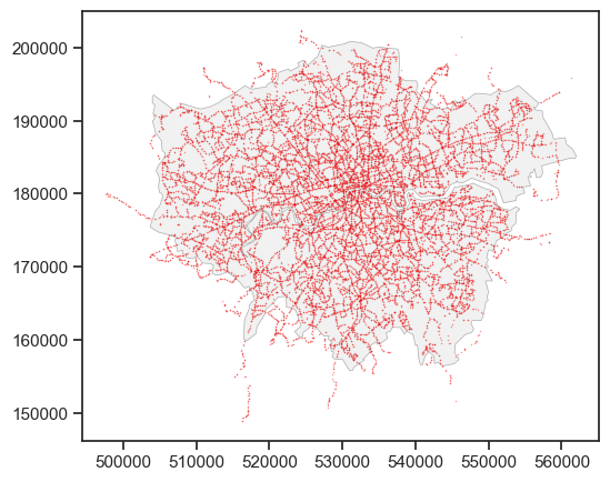
A dot map can be used to visualize the distribution of the point data. The dot map can directly show the density of the locations for a large number of points.

# Read the TfL Bus Stop Locations data
df_bus_stop = pd.read_csv("data/tfl_bus-stops.csv")

# Convert the DataFrame to a GeoDataFrame
gdf_bus_stop = gpd.GeoDataFrame(df_bus_stop, geometry=gpd.points_from_xy(df_bus_stop['Location_Easting'], df_bus_stop['Location_Northing']))

# We also need the London boundary (we create this boundary by dissolve function in last week) to add the background of the map.
gdf_london_boundary = gpd.read_file("data/whole_london_boundary.geojson")
# transfer the coordinate system of the London boundary to OSGB36
gdf_london_boundary = gdf_london_boundary.to_crs("EPSG:27700")

# Plot the bus stops and London boundary on a map
# Create a figure and axis
fig, ax = plt.subplots(figsize=(6, 6))
# Plot the London boundary
gdf_london_boundary.plot(ax=ax, # ax is the axis to plot on
                          color='lightgrey', # color of the polygon
                          edgecolor='black', # color of the boundary
                          alpha=0.3, # transparency of all colors
                          linewidth=0.5) # linewidth of the polygon boundary
# The bus stop points plot
gdf_bus_stop.plot(ax=ax, # another layer of points but put in the same axis
                  color='red', # color of the points
                  edgecolor='grey',  # color of the point boundary
                  linewidth=0.05, # linewidth of the point boundary
                  markersize=1, # size of the points
                  alpha=0.4, # transparency of the all colors
                  label='TfL Bus Stops', # label of the points
                   )
# We need the matplotlib_map_utils to add the scale bar and north arrow on the map
from matplotlib_map_utils.core.north_arrow import NorthArrow, north_arrow
from matplotlib_map_utils.core.scale_bar import ScaleBar, scale_bar
NorthArrow.set_size("small")
ScaleBar.set_size("small")
# Add the North Arrow and scale bar to the map
north_arrow(ax, location="upper right", rotation={"crs": gdf_bus_stop.crs, "reference": "center"})
scale_bar(ax, location="upper left", style="boxes", bar={"projection": gdf_bus_stop.crs})
# Set the title
ax.set_title('TfL Bus Stops in London')
# Set the legend
ax.legend(labels=['Bus Stops Locations'], loc='lower left', fontsize=8)
ax.set_xlabel('Easting (m)')
ax.set_ylabel('Northing (m)')
# We can save the figure as a jpg file
# plt.savefig("tfl_bus_stops.jpg", dpi=300, bbox_inches='tight')
plt.show()

---------------------------------------------------------------------------
ValueError                                Traceback (most recent call last)
Cell In[5], line 25
     23 ScaleBar.set_size("small")
     24 # Add the North Arrow and scale bar to the map
---> 25 north_arrow(ax, location="upper right", rotation={"crs": gdf_bus_stop.crs, "reference": "center"})
     26 scale_bar(ax, location="upper left", style="boxes", bar={"projection": gdf_bus_stop.crs})
     27 # Set the title

File ~/PycharmProjects/MSc_AI_DS_Research_Projects/.venv/lib/python3.11/site-packages/matplotlib_map_utils/core/north_arrow.py:287, in north_arrow(ax, draw, location, scale, base, fancy, label, shadow, pack, aob, rotation)
    285 _pack = naf._validate_dict(pack, _DEFAULT_PACK, nat._VALIDATE_PACK, return_clean=True)
    286 _aob = naf._validate_dict(aob, _DEFAULT_AOB, nat._VALIDATE_AOB, return_clean=True)
--> 287 _rotation = naf._validate_dict(rotation, _DEFAULT_ROTATION, nat._VALIDATE_ROTATION, return_clean=True)
    289 # First, getting the figure for our axes
    290 fig = ax.get_figure()

File ~/PycharmProjects/MSc_AI_DS_Research_Projects/.venv/lib/python3.11/site-packages/matplotlib_map_utils/validation/functions.py:243, in _validate_dict(input_dict, default_dict, functions, to_validate, return_clean, parse_false)
    241 # NOTE: This is messy but the only way to get the rotation value to the crs function
    242 if key=="crs":
--> 243     _ = func(prop=key, val=val, rotation_dict=values, **fd["kwargs"])
    244 # NOTE: This is messy but the only way to check the projection dict without keywords
    245 elif key=="projection":

File ~/PycharmProjects/MSc_AI_DS_Research_Projects/.venv/lib/python3.11/site-packages/matplotlib_map_utils/validation/functions.py:101, in _validate_crs(prop, val, rotation_dict, none_ok)
     99 if reference == "center":
    100     if crs is None:
--> 101         raise ValueError(f"If degrees is set to None, and reference is 'center', then a valid crs must be supplied")
    102 else:
    103     if crs is None or reference is None or coords is None:

ValueError: If degrees is set to None, and reference is 'center', then a valid crs must be supplied

Tailoring the dot map

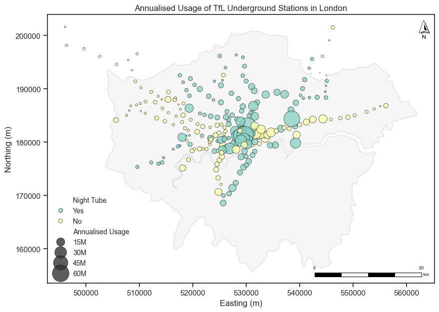
We can tailor the dot map by changing the size of the dots, the color of the dots, and the transparency of the dots according to different attributes of the data (e.g., categorical data and numerical data).

• Different colors represent different categories of the data (e.g., different types of transport).

• Different sizes represent different values of the data (e.g., population size).

# Read the TfL Underground station geo-data
gdf_underground = gpd.read_file("data/Underground_Stations.geojson")
# transfer the coordinate system of the Underground stations to OSGB36
gdf_underground = gdf_underground.to_crs("EPSG:27700")
gdf_underground

	OBJECTID	NAME	LINES	ATCOCODE	MODES	ACCESSIBILITY	NIGHT_TUBE	NETWORK	DATASET_LAST_UPDATED	FULL_NAME	geometry
0	111	St. Paul's	Central	940GZZLUSPU	bus, tube	Not Accessible	Yes	London Underground	2021-11-29 00:00:00+00:00	St. Paul's station	POINT Z (532110.145 181274.419 0)
1	112	Mile End	District, Hammersmith & City, Central	940GZZLUMED	bus, tube	Partially Accessible - Interchange Only	Yes	London Underground	2021-11-29 00:00:00+00:00	Mile End station	POINT Z (536502.678 182534.693 0)
2	113	Bethnal Green	Central	940GZZLUBLG	bus, tube	Not Accessible	Yes	London Underground	2021-11-29 00:00:00+00:00	Bethnal Green station	POINT Z (535045.414 182718.596 0)
3	114	Leyton	Central	940GZZLULYN	bus, tube	Not Accessible	Yes	London Underground	2021-11-29 00:00:00+00:00	Leyton station	POINT Z (538369.354 186076.113 0)
4	115	Snaresbrook	Central	940GZZLUSNB	bus, tube	Not Accessible	Yes	London Underground	2021-11-29 00:00:00+00:00	Snaresbrook station	POINT Z (540158.622 188804.247 0)
...	...	...	...	...	...	...	...	...	...	...	...
268	483	Seven Sisters	Victoria	940GZZLUSVS	tube	Not Accessible	Yes	London Underground	2021-11-29 00:00:00+00:00	Seven Sisters station	POINT Z (533644.648 188931.178 0)
269	484	Theydon Bois	Central	940GZZLUTHB	tube	Partially Accessible	No	London Underground	2021-11-29 00:00:00+00:00	Theydon Bois station	POINT Z (545543.329 199101.251 0)
270	485	Kenton	Bakerloo	940GZZLUKEN	tube	Not Accessible	No	London Underground	2021-11-29 00:00:00+00:00	Kenton station	POINT Z (516729.561 188314.716 0)
271	486	Woodside Park	Northern	940GZZLUWOP	tube, bus	Fully Accessible	No	London Underground	2021-11-29 00:00:00+00:00	Woodside Park station	POINT Z (525720.193 192588.5 0)
272	487	Preston Road	Metropolitan	940GZZLUPRD	tube, bus	Not Accessible	No	London Underground	2021-11-29 00:00:00+00:00	Preston Road station	POINT Z (518250.918 187282.096 0)

273 rows × 11 columns

We will add usage information (counted by entry/exit) of London Underground stations to build a dot map. The usage data was published by TfL in the London Underground Station Crowding page. The usage data is in the CSV or XLSX format, and we can read it using the Pandas library.

# we only need the London Underground stations and annualised usage, so we need to filter the data.
df_usage_lu = df_usage[df_usage['Unnamed: 0'] == 'LU'][['Unnamed: 3', 'Annualised']].rename(columns={'Unnamed: 3': 'name', 'Annualised': 'usage'})
df_usage_lu.head()

	name	usage
1	Acton Town	4823835
2	Aldgate	6897314
3	Aldgate East	10947896
4	Alperton	2598605
5	Amersham	1729521

# Note that the usage columns have some missing values and some values are string '---' which means no data.
# You can use more codes to fill the data as NaN occurs as the mismatch of the name between the two datasets, though some cases are indicating one station.
print(gdf_underground_usage.usage.values)

[9189088 11145822 nan 8592536 1849887 6955728 1948236 4051381 3371643
 1167037 885823 4492296 267679 332284 nan 4383503 8491273 10787392 806675
 1503305 3937018 1212120 2153159 1860607 6314434 3063800 1597432 6030683
 6258859 1631696 1555062 1663555 1654538 2598605 4159381 13568222 27379635
 12573815 7822836 5106522 2203557 3293586 3947509 1450247 2307306 5962575
 7049636 nan 4377539 nan 14965619 6897314 nan 23330204 5185508 40070382
 72124262 11239346 21207073 nan nan 3644937 9413060 11353518 26088906
 2074444 1841679 5785361 3763523 5568858 7890670 nan 2624208 2899358 nan
 nan 7087668 nan 14076462 2645552 2542830 1623305 838918 3216718 1804676
 1952034 5748997 2138577 15779710 4373423 12110869 3172252 8590075
 37424555 1722368 3269238 5652447 5008989 nan 51106043 20240977 7803444
 9576731 6802053 nan 23172392 12328817 5573360 nan 5236551 7045026 5339416
 7137484 12397420 6265211 6323510 8040059 5210928 5113576 58726155 3889479
 2967011 4532637 '---' 4875982 5615724 4633070 3130908 1604937 1455300
 4909025 14142708 8975412 nan 6151983 1786001 2752421 2861021 397280
 1841035 3276268 2005688 3043893 3466311 3061427 820575 3540050 2385943
 17051267 2042489 1817060 2466317 4598994 1296040 nan 3937317 4045767
 26739879 nan nan 2689160 nan 2681574 2617813 nan 2297814 13156281 2717311
 nan 5022937 9088053 4266560 19172572 '---' nan nan 4774045 5338957
 13349683 15429088 4823835 1954910 28247401 20479785 7381051 8263631 nan
 2852360 2776023 3000487 3370726 1675267 2782422 5240900 6823150 5181211
 2134593 4663306 10947896 17452196 4157626 15510977 2565708 1989399 nan
 1057631 54376225 5419509 1373730 853803 1463521 1396078 1408690 1003523
 3340365 1398638 2223811 8435460 3353641 3002979 2073359 5870213 8508705
 nan 11223888 1296777 8399835 4108613 4040066 605628 4354076 nan 5347065
 4731235 4827763 nan 3529781 2547324 4780369 3727656 8875310 3019402
 9534074 7948900 15137045 3609039 1435853 5133701 3259745 2158123 1729521
 5426495 nan 18805872 nan 4321012 5198096 4408040 966889 1851241 808774
 2162088 837496 1653584 4067823 15846905 12258814 5179915 12165434 734300
 1515511 3657219 2423452]

# Plot the Underground stations with usage data
# Create a figure and axis
fig, ax = plt.subplots(figsize=(8, 8))
# Plot the London boundary
gdf_london_boundary.plot(ax=ax, # ax is the axis to plot on
                          color='lightgrey', # color of the polygon
                          edgecolor='black', # color of the boundary
                          alpha=0.2, # transparency of all colors
                          linewidth=0.5) # linewidth of the polygon boundary
# The Underground stations plot
gdf_underground_usage_s.plot(ax=ax,
                     column='usage', # column name to tailor the dot map, here is the numerical data
                     cmap='viridis', # color map
                      markersize=40, # size of the points
                      alpha=0.7, # transparency of the all colors
                      edgecolor='black', # color of the point boundary
                      linewidth=0.5, # linewidth of the point boundary
                      legend=True,
                      legend_kwds={ "label": "Annualised Usage",
                                    "orientation": "horizontal"
                                    },
                      )
# Add the North Arrow and scale bar to the map
north_arrow(ax, location="upper right", rotation={"crs": gdf_underground.crs, "reference": "center"})
scale_bar(ax, location="lower left", style="boxes", bar={"projection": gdf_underground.crs})
# Set the title
ax.set_title('Annualised Usage of TfL Underground Stations in London')
ax.set_xlabel('Easting (m)')
ax.set_ylabel('Northing (m)')
plt.show()

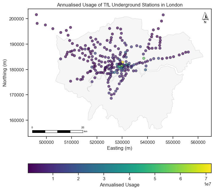
A proportional map is a variation of a dot map, where the size of the dots is proportional to the value of the variable being represented.

# Plot the Underground stations with usage data
# Create a figure and axis
fig, ax = plt.subplots(figsize=(10, 10))
# Plot the London boundary
gdf_london_boundary.plot(ax=ax, # ax is the axis to plot on
                          color='lightgrey', # color of the polygon
                          edgecolor='black', # color of the boundary
                          alpha=0.2, # transparency of all colors
                          linewidth=0.5) # linewidth of the polygon boundary
# We use the seaborn to plot the Underground stations
sns.scatterplot(ax=ax,
                data=gdf_underground_usage_s,
                x=gdf_underground_usage_s.geometry.x, # x coordinate
                y=gdf_underground_usage_s.geometry.y, # y coordinate
                hue='NIGHT_TUBE', # column name to tailor the dot map, here is the categorical data
                size=gdf_underground_usage_s['usage'], # size of the points
                sizes=(0, 700), # size range of the point selection
                alpha=0.8, # transparency of the all colors
                palette='Set3', # color map
                linewidth=0.5, # linewidth of the point boundary
                edgecolor='black', # color of the point boundary
                legend=True,
                 )
# Add the North Arrow and scale bar to the map
north_arrow(ax, location="upper right", rotation={"crs": gdf_london_boundary.crs, "reference": "center"})
scale_bar(ax, location="lower right", style="boxes", bar={"projection": gdf_london_boundary.crs})
# Set the legend
handles, labels = ax.get_legend_handles_labels()
ax.legend(handles=handles,
          labels=['Night Tube', 'Yes', 'No', 'Annualised Usage', '15M', '30M', '45M', '60M'],
          loc='lower left', fontsize=10, title_fontsize=12, frameon=False)
# Set the title
ax.set_title('Annualised Usage of TfL Underground Stations in London')
ax.set_xlabel('Easting (m)')
ax.set_ylabel('Northing (m)')
plt.show()

A choropleth map is a type of thematic map where areas are shaded or patterned in proportion to the value of a variable being represented. It is used to visualize the spatial distribution of a variable across different regions (Polygons).

# Read the UK LAs data
gdf_las = gpd.read_file("data/Local_Authority_Districts_December_2024_Boundaries_UK_BSC.geojson")
# Convert the coordinate reference system (CRS) to OSGB
gdf_las = gdf_las.to_crs("EPSG:27700")
gdf_las['area'] = gdf_las.geometry.area / 1e6 # convert the area to km2

# Read the 2022 population data
df_pop = pd.read_csv("data/populaiton_2022_all_ages_uk.csv")

# merge the population data with the gdf_las data
gdf_las_pop = pd.merge(gdf_las, df_pop, left_on='LAD24CD', right_on='Code', how='left')
gdf_las_pop = gdf_las_pop.rename(columns={'All ages': 'population'})
# calculate the population density
gdf_las_pop['density'] = gdf_las_pop['population'] / gdf_las_pop['area'] # calculate the population density

We have used a sequential color to plot the population distribution across the UK LAs. The darker the color, the higher the population. Alternatively, we can change the legend which means we can use the categorical data to plot the choropleth map. For example, we can classify the population density to several levels and plot the choropleth map by using setting scheme and k in the plot().

import contextily as cx

Interactive maps are maps that allow users to interact with the map by zooming, panning, and clicking on features. They are used to visualize geospatial data in a more dynamic way. There are several libraries in Python that can be used to create interactive maps, such as Folium, Plotly, and Bokeh. You can find an interactive map of uk LA population density generated from the Folium at here (click).

import libpysal
import spreg
# ensure the spreg pkg is at least the 1.8.2 version
print(spreg.__version__)

1.8.3

A spatial weight matrix (spatial adjacency matrix) \(W\) is a square matrix that quantifies the spatial relationship between each pair of locations (i and j are the spatial unit index) across \(n\) spatial units: $$ W =

(1)\[\begin{bmatrix} w_{11} & w_{12} & \dots & w_{1n} \\ w_{21} & w_{22} & \dots & w_{2n} \\ \vdots & \vdots & \ddots & \vdots \\ w_{n1} & w_{n2} & \dots & w_{nn} \end{bmatrix}\]

\[ \begin{align}\begin{aligned}- $w_{ij}$ is the spatial weight between location $i$ and $j$; - Typically, $w_{ii} = 0$ (no self-weight).\\For example, if we have 4 areas/locations (A, B, C, D) with the index (1, 2, 3, 4) and the following spatial weight matrix can be $W$: \end{aligned}\end{align} \]

W =

(2)\[\begin{bmatrix} w_{11} & w_{12} & w_{13} & w_{14} \\ w_{21} & w_{22} & w_{23} & w_{24} \\ w_{31} & w_{32} & w_{33} & w_{34} \\ w_{41} & w_{42} & w_{43} & w_{44} \end{bmatrix}\]

$$

• pysal library community consist lots of pkgs in spatial analysis, like spreg, esda, libpysal and mgwr.

• NYC Neighborhoods Data Page

gdf_nyc.crs

<Geographic 2D CRS: EPSG:4326>
Name: WGS 84
Axis Info [ellipsoidal]:
- Lat[north]: Geodetic latitude (degree)
- Lon[east]: Geodetic longitude (degree)
Area of Use:
- name: World.
- bounds: (-180.0, -90.0, 180.0, 90.0)
Datum: World Geodetic System 1984 ensemble
- Ellipsoid: WGS 84
- Prime Meridian: Greenwich

import libpysal.weights as weights

df_wq = w_q.to_adjlist(drop_islands=True)
df_wq

	focal	neighbor	weight
0	0	17	1.0
1	0	31	1.0
2	0	77	1.0
3	0	155	1.0
4	1	17	1.0
...	...	...	...
1085	194	22	1.0
1086	194	38	1.0
1087	194	79	1.0
1088	194	94	1.0
1089	194	139	1.0

1090 rows × 3 columns

More usages can be found at The libysal function page

Global spatial autocorrelation:

Global spatial autocorrelation answers the question: Is there overall clustering across the whole map?

Moran’s I (Moran, 1950) is a measure of global spatial autocorrelation. It is a single value that summarizes the degree of spatial autocorrelation in the entire dataset: $\( I = \frac{n}{W} \cdot \frac{\sum_i \sum_j w_{ij} (x_i - \bar{x})(x_j - \bar{x})}{\sum_i (x_i - \bar{x})^2} \)$

Where:

• \( n \): Number of spatial units

• \( x_i \): Value at location \( i \)

• \( \bar{x} \): Mean of the variable

• \( w_{ij} \): Spatial weight between location \( i \) and \( j \)

• \( W = \sum_i \sum_j w_{ij} \): Sum of all spatial weights

\(I > 0\): Positive spatial autocorrelation.

\(I < 0\): Negative spatial autocorrelation.

\(I = 0\): No spatial autocorrelation.

# compute the global Moran's I for total population
import esda
gdf_nyc['poptot'] = gdf_nyc['poptot'].astype(int)
mi = esda.Moran(gdf_nyc['poptot'], w_q, two_tailed=True)

Local spatial autocorrelation:

Local spatial autocorrelation answers the questions: Is there clustering in a specific area? Which specific areas are clustered or are spatial outlier?

Local indicators of spatial association (LISA):

is a statistical technique that decomposes global spatial autocorrelation measures into location-specific contributions. It identifies significant spatial clusters or spatial outliers by measuring the correlation between a location and its neighbors.

• Local Moran’s I:

Local Moran’s I is a measure of local spatial autocorrelation. It is a value for each spatial unit that summarizes the degree of spatial autocorrelation in the local neighborhood of that unit: $\( I_i = \frac{(x_i - \bar{x})}{S^2} \cdot \sum_j w_{ij} (x_j - \bar{x}) \)$

Where:

• \( I_i \): Local Moran’s I for location \( i \)

• \( x_i \): Value at location \( i \)

• \( \bar{x} \): Mean of the variable

• \( S\): Standard deviation of the variable

• \( S^2 \): Variance of the variable

• \( w_{ij} \): Spatial weight between location \( i \) and \( j \)

• \( j \): Neighbors of location \( i \)

• \( \sum_j w_{ij} \): Sum of the spatial weights for location \( i \)

\( I_i > 0 \): Positive spatial autocorrelation (high values surrounded by high values or low values surrounded by low values)

\(I_i < 0 \): Negative spatial autocorrelation (high values surrounded by low values or low values surrounded by high values)

\(I_i = 0 \): No spatial autocorrelation You can find etails about the Local Moran’s I in the libpysal Local Moran I documentation.

• Getis-Ord Gi*:

Gi* is a measure of local spatial autocorrelation that identifies clusters of high or low values. It is similar to Local Moran’s I, but it is more sensitive to the presence of outliers. It is used to identify hot spots (high values) and cold spots (low values) in the data: $\( G_i^* = \frac{\sum_j w_{ij} (x_j - \bar{x})}{\sqrt{\frac{S^2}{n}}} \)$ Where:

• \( G_i^* \): Getis-Ord Gi* for location \( i \);

• \( x_i \): Value at location \( i \);

• \( \bar{x} \): Mean of the variable;

• \( S^2 \): Variance of the variable;

• \( n \): Number of spatial units;

• \( w_{ij} \): Spatial weight between location \( i \) and \( j \);

• \( j \): Neighbors of location \( i \);

• \( \sum_j w_{ij} \): Sum of the spatial weights for location \( i \);

• \( \sqrt{\frac{S^2}{n}} \): Standard deviation of the variable;

• \( \sum_j w_{ij} \): Sum of the spatial weights for location \( i \);

• \( \sqrt{\frac{S^2}{n}} \): Standard deviation of the variable;

• \( \sum_j w_{ij} \): Sum of the spatial weights for location \( i \).

Z-scores: standardized G statistics that follow a normal distribution under spatial randomness.

P values: P-values from randomization/permutation.

You can use any strategies to plot the gi resluts, here we can plot the results to the map with three parts:

• Hotspots: High positive Z-score (>0) with p-value < 0.05.

• Coldspots: High negative Z-score (<0) with p-value < 0.05.

• We usually use blank color to draw the ‘Not Significant cluster’ (p_value \(\geq\) 0.05).

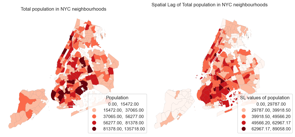
2.2.3 Spatial lags

# we can use the libpysal to compute the spatial lag
import libpysal as lps
ylag = lps.weights.lag_spatial(w_q, gdf_nyc['poptot'])
print(ylag)

[49362.25       28475.         47006.375      51427.75
 33904.33333333 29394.         16276.33333333 30615.83333333
 24442.6        26460.66666667 36855.4        35909.16666667
 16313.5        25859.66666667 32423.         24938.33333333
 35500.         51096.18518519 38548.04166667 27779.4
 42008.25       48425.66666667 40841.52631579 32608.25
 29787.         47603.33333333 29392.6        89058.
 39918.5            0.         43581.375      56055.6
 21846.75       32732.5        48332.8        27345.
 26674.83333333 33253.75       41449.         29378.5
 41864.14285714 33103.         22970.6        46351.
 49333.8        30433.11111111 31618.75       40978.16666667
 49566.2        17969.         21665.         46341.33333333
 57367.76470588 27424.44444444 26972.33333333 37355.22222222
 47931.6        39146.5        53198.         70978.375
 32600.4        38980.25       28301.42857143 30198.
 36467.5        56681.25       32198.         32485.4
 73155.2        66668.66666667 29724.57142857 46159.
 25791.5        34756.875      57186.6        28039.28571429
 33982.42857143 45772.66666667 57685.         35781.75
 45147.6        33185.33333333 60449.         26227.25
 58117.6        52577.33333333 56311.6        56218.
 23641.33333333 31126.4        42913.33333333 39061.6
 23819.         39723.33333333 54064.66666667 35346.4
 56398.8        24372.         39252.8        58900.2
 44591.875      22039.25       46541.         35084.4
 37563.5        35568.57142857 31351.5        24651.75
 55706.         61634.33333333 35926.         33531.28571429
 38671.33333333 43120.66666667 32351.16666667 42640.125
 38910.375      52090.         34730.         46812.
 37278.6        48268.         29281.5        29394.
 42948.16666667 46641.         41365.         27143.
 51776.4        56350.66666667 24468.16666667 24628.
 26826.         49325.         32260.5        42973.6
 68325.75       44167.28571429 32440.         53287.6
 26728.5        36147.57142857 44762.5        37229.8
 32338.         29262.2        28446.         30908.
 54011.25       55331.5        55481.4        53901.
 58571.         47130.66666667 31085.5        62864.85714286
 32366.5        26322.66666667 75716.         32316.5
 38722.4        15612.5        37183.4        37630.
 39275.85714286 43798.66666667 62967.16666667 41816.66666667
 36007.8        40267.         45930.3        52549.6
 48399.4        49492.         49030.4        46985.85714286
 44372.         26605.75       28592.14285714 26234.83333333
 22638.         29548.42857143 23352.         29178.
 65779.42857143 62009.6        47940.4        24141.5
 27331.4        32973.875      48749.         53538.2
 44769.71428571 52693.2        33380.33333333]

# Plot the original data and spatial lag of the population data for comparison
fig, ax = plt.subplots(1, 2, figsize=(12, 8))
gdf_nyc.plot(column='poptot', ax=ax[0], legend=True, cmap='Reds',
                       edgecolor='black', linewidth=0.05, scheme = 'naturalbreaks',
                       legend_kwds = {'bbox_to_anchor': (1.2, 0.35),'title': "Population"})
ax[0].set_title('Total population in NYC neighbourhoods')

gdf_nyc.plot(column='sl_poptop', ax=ax[1], legend=True, cmap='Reds',
                       edgecolor='black', linewidth=0.05, scheme = 'naturalbreaks',
                       legend_kwds = {'bbox_to_anchor': (1.2, 0.35),'title': "SL values of population"})
ax[1].set_title('Spatial Lag of Total population in NYC neighbourhoods')
ax[0].set_axis_off()
ax[1].set_axis_off()
plt.show()

The Spatial Lag Model (SLM) is a type of regression model that explicitly includes the effect of neighboring dependent variable values (i.e., spatial lag) on the value at each location:

\[ \mathbf{y} = \rho \mathbf{W y} + \mathbf{X} \boldsymbol{\beta} + \boldsymbol{\epsilon} \]

• \(\mathbf{y}\) is the vector of the dependent variable

• \(\mathbf{W}\) is the spatial weights matrix, so \(\mathbf{W y}\) is the spatial lag of \(\mathbf{y}\)

• \(\rho\) is the spatial autoregressive coefficient

• \(\mathbf{X}\) is the matrix of explanatory variables

• \(\boldsymbol{\beta}\) is the vector of coefficients

• \(\boldsymbol{\epsilon}\) is the error term

# we need to set the crs to EPSG:26917 (NAD83 / UTM zone 17N) as the polygon valus in the data is in this CRS, not the EPSG:4326.
gdf_columbus = gdf_columbus.set_crs(epsg=26917, allow_override=True)
print(gdf_columbus.crs)

EPSG:26917

# Spatial weights
w = weights.Queen.from_dataframe(gdf_columbus, use_index='True')
w.transform = 'R'  # Row-standardized

# Variables
y = gdf_columbus[['CRIME']].values          # Dependent variable
X = gdf_columbus[['INC', 'HOVAL']].values   # Independent variables are Income and House Value.

# Fit spatial lag model
model_sl = ML_Lag(y, X, w=w, name_y='CRIME', name_x=['INC', 'HOVAL'], name_w='Queen', name_ds='Columbus')

# Output summary
print(model_sl.summary)

REGRESSION RESULTS
------------------

SUMMARY OF OUTPUT: MAXIMUM LIKELIHOOD SPATIAL LAG (METHOD = FULL)
-----------------------------------------------------------------
Data set            :    Columbus
Weights matrix      :       Queen
Dependent Variable  :       CRIME                Number of Observations:          49
Mean dependent var  :     35.1288                Number of Variables   :           4
S.D. dependent var  :     16.7321                Degrees of Freedom    :          45
Pseudo R-squared    :      0.6473
Spatial Pseudo R-squared:  0.5806
Log likelihood      :   -182.6740
Sigma-square ML     :     96.8572                Akaike info criterion :     373.348
S.E of regression   :      9.8416                Schwarz criterion     :     380.915

------------------------------------------------------------------------------------
            Variable     Coefficient       Std.Error     z-Statistic     Probability
------------------------------------------------------------------------------------
            CONSTANT        45.60325         7.25740         6.28369         0.00000
                 INC        -1.04873         0.30741        -3.41154         0.00065
               HOVAL        -0.26633         0.08910        -2.98929         0.00280
             W_CRIME         0.42333         0.11951         3.54216         0.00040
------------------------------------------------------------------------------------

SPATIAL LAG MODEL IMPACTS
Impacts computed using the 'simple' method.
            Variable         Direct        Indirect          Total
                 INC        -1.0487         -0.7699         -1.8186
               HOVAL        -0.2663         -0.1955         -0.4618
================================ END OF REPORT =====================================

In summary, the results reflect the spatial lag model equation, where the spatial autoregressive coefficient \(\rho\) corresponds to the coefficient of W_CRIME (0.42). The vector of regression coefficients \(\boldsymbol{\beta}\) includes the coefficients for INC and HOVAL, which are -1.05 and -0.27 respectively. The error term \(\boldsymbol{\epsilon}\) is represented by the standard error of the regression (9.84) and the maximum likelihood estimate of the error variance (Sigma-square ML = 96.86).

residuals = model_sl.u  # residuals from the SLM
moran_resid = esda.Moran(residuals, w)
print(moran_resid.I, moran_resid.p_sim)

0.033068305761995494 0.268

# get the in sample prediction (fttted) crime rates and the residuals
gdf_columbus["fitted"] = model_sl.predy.flatten()
gdf_columbus["residuals"] = model_sl.u.flatten()

2.2.5 Spatial Durbin Model (SDM)

The Spatial Durbin Model (SDM) is specified as:

\[ \mathbf{y} = \rho \mathbf{W} \mathbf{y} + \mathbf{X} \boldsymbol{\beta} + \mathbf{W} \mathbf{X} \boldsymbol{\theta} + \boldsymbol{\varepsilon} \]

where:

• \( \mathbf{y} \) is the dependent variable vector,

• \( \rho \mathbf{W} \mathbf{y} \) represents the spatial lag of the dependent variable,

• \( \mathbf{X} \boldsymbol{\beta} \) are the usual covariates,

• \( \mathbf{W} \mathbf{X} \boldsymbol{\theta} \) are the spatially lagged covariates,

• \( \boldsymbol{\varepsilon} \sim \mathcal{N}(0, \sigma^2 \mathbf{I}) \) is the error term.

# Fit spatial lag model
model_dur = ML_Lag(y, X, w=w, name_y='CRIME', name_x=['INC', 'HOVAL'], name_w='Queen', name_ds='Columbus',
                   slx_lags=1,
                   slx_vars= [True, True])

# Output summary
print(model_dur.summary)

REGRESSION RESULTS
------------------

SUMMARY OF OUTPUT: MAXIMUM LIKELIHOOD SPATIAL LAG WITH SLX - SPATIAL DURBIN MODEL (METHOD = FULL)
-------------------------------------------------------------------------------------------------
Data set            :    Columbus
Weights matrix      :       Queen
Dependent Variable  :       CRIME                Number of Observations:          49
Mean dependent var  :     35.1288                Number of Variables   :           6
S.D. dependent var  :     16.7321                Degrees of Freedom    :          43
Pseudo R-squared    :      0.6603
Spatial Pseudo R-squared:  0.6120
Log likelihood      :   -181.6393
Sigma-square ML     :     93.2722                Akaike info criterion :     375.279
S.E of regression   :      9.6578                Schwarz criterion     :     386.629

------------------------------------------------------------------------------------
            Variable     Coefficient       Std.Error     z-Statistic     Probability
------------------------------------------------------------------------------------
            CONSTANT        44.32001        13.04547         3.39735         0.00068
                 INC        -0.91991         0.33474        -2.74811         0.00599
               HOVAL        -0.29713         0.09042        -3.28625         0.00102
               W_INC        -0.58391         0.57422        -1.01687         0.30921
             W_HOVAL         0.25768         0.18723         1.37626         0.16874
             W_CRIME         0.40346         0.16133         2.50079         0.01239
------------------------------------------------------------------------------------

DIAGNOSTICS FOR SPATIAL DEPENDENCE
TEST                              DF         VALUE           PROB

SPATIAL DURBIN MODEL IMPACTS
Impacts computed using the 'simple' method.
            Variable         Direct        Indirect          Total
                 INC        -0.9199         -1.6010         -2.5209
               HOVAL        -0.2971          0.2310         -0.0661
================================ END OF REPORT =====================================

Geographically Weighted Regression (GWR) and Multiscale Geographically Weighted Regression (MGWR) model can be found at here(click)

Machine learning (ML) workflow

ML tasks in space and time

2.3.1 SVM regression model and hyperpramer using GridSearch + Random CV

Step 1 Problem definition:

We will use the POI data (X features) to predict the crime levels (y targets) across London grids (1km and 1km) via the machine learning models.

# Load the house price data
gdf_grid = gpd.read_file('data/GEOSTAT_Dec_2011_GEC_in_the_United_Kingdom_2022.geojson')
gdf_grid.head()

	OBJECTID	grd_fixid	grd_floaid	grd_newid	pcd_count	tot_p	tot_m	tot_f	tot_hh	GlobalID	geometry
0	1	4.0.31510000.31050000	3151.3105.4	1kmN3105E3151	0	0	0	0	0	c142c42b-5160-4760-a836-956a3920caf8	POLYGON ((-6.41829 49.87519, -6.41852 49.87527...
1	2	4.0.31520000.31040000	3152.3104.4	1kmN3104E3152	0	0	0	0	0	26709ad2-2ae8-4f76-95f4-850c60e9c8e6	POLYGON ((-6.41461 49.87373, -6.40491 49.87515...
2	3	4.0.31520000.31050000	3152.3105.4	1kmN3105E3152	0	0	0	0	0	e477a513-48a2-4012-9cd7-3063ac2bc6c6	POLYGON ((-6.40698 49.8838, -6.40414 49.87568,...
3	4	4.0.31520000.31060000	3152.3106.4	1kmN3106E3152	0	0	0	0	0	8d1562d5-3252-40ef-858e-c80391bebefe	POLYGON ((-6.40726 49.88398, -6.42047 49.88204...
4	5	4.0.31530000.31050000	3153.3105.4	1kmN3105E3153	0	0	0	0	0	2952357c-da71-4e17-93a0-ace5e73e86d4	POLYGON ((-6.40414 49.87568, -6.40698 49.8838,...

# read the London boundary
gdf_london_bound = gpd.read_file('data/whole_london_boundary.geojson')
# to select the Grids in London, we do not use the overlay to clip the shap but use the spatial join to select the grids of London
gdf_london_grid = gpd.sjoin(gdf_grid, gdf_london_bound, how='inner', predicate='intersects')

# drop the index_right column
gdf_london_grid = gdf_london_grid.drop(columns=['index_right'])

# here we only use the gis_osm_pois_free_1.shp file
gdf_poi = gpd.read_file('data/osm_england-latest-free-shp/gis_osm_pois_free_1.shp')
gdf_poi.columns

Index(['osm_id', 'code', 'fclass', 'name', 'geometry'], dtype='object')

# we calculate the numbers and poi type for each grid
df_poi_counts = gdf_poi_grid_s.groupby(['grd_newid']).size().reset_index(name='poi_counts')
df_poi_types = gdf_poi_grid_s.groupby(['grd_newid']).nunique()['fclass'].reset_index(name='poi_types')

# read the crime data
df_crime = pd.read_csv('data/crime_2024_call_police_met_city.csv')
# transfer df to gdf
gdf_crime_s = gpd.GeoDataFrame(df_crime, geometry=gpd.points_from_xy(df_crime['Longitude'], df_crime['Latitude']), crs='EPSG:4326')

# merge the crime data with the grid data
gdf_london_grid_poi_crime = gdf_poi_grid_s_poi_type.merge(df_crime, on='grd_newid', how='left')
# gdf_london_grid_poi_crime.to_file('data/london_grid_poi_crime.geojson', driver='GeoJSON')

Step 3 Data Splitting:

Step 4 Feature Scaling:

Step 5 Model Training and Hyperparameter Tuning (Cross-Validation):

Random CV and GridSearch

gscv_results_df = pd.DataFrame(grid_search.cv_results_)
gscv_results_df

	mean_fit_time	std_fit_time	mean_score_time	std_score_time	param_C	param_epsilon	param_gamma	param_kernel	params	split0_test_score	split1_test_score	split2_test_score	split3_test_score	split4_test_score	mean_test_score	std_test_score	rank_test_score
0	0.011516	0.001450	0.002091	0.000071	0.1	0.1	scale	linear	{'C': 0.1, 'epsilon': 0.1, 'gamma': 'scale', '...	-0.161602	-0.309483	-0.269594	-0.213100	-1.038503	-0.398456	0.323925	39
1	0.012661	0.000412	0.004879	0.000386	0.1	0.1	scale	rbf	{'C': 0.1, 'epsilon': 0.1, 'gamma': 'scale', '...	-0.178756	-0.425421	-0.337690	-0.235625	-1.408892	-0.517277	0.453782	119
2	0.046547	0.011293	0.001759	0.000071	0.1	0.1	scale	poly	{'C': 0.1, 'epsilon': 0.1, 'gamma': 'scale', '...	-0.235991	-0.381201	-0.431818	-0.278688	-0.515603	-0.368660	0.101424	6
3	0.010931	0.000872	0.001876	0.000066	0.1	0.1	auto	linear	{'C': 0.1, 'epsilon': 0.1, 'gamma': 'auto', 'k...	-0.161602	-0.309483	-0.269594	-0.213100	-1.038503	-0.398456	0.323925	39
4	0.012968	0.002267	0.004626	0.000337	0.1	0.1	auto	rbf	{'C': 0.1, 'epsilon': 0.1, 'gamma': 'auto', 'k...	-0.179099	-0.424231	-0.337557	-0.236367	-1.408735	-0.517198	0.453636	118
...	...	...	...	...	...	...	...	...	...	...	...	...	...	...	...	...	...
139	0.022242	0.002893	0.002663	0.000720	100.0	0.3	0.1	rbf	{'C': 100, 'epsilon': 0.3, 'gamma': 0.1, 'kern...	-0.189447	-0.327770	-0.273917	-0.211199	-1.403278	-0.481122	0.463628	97
140	0.115625	0.023100	0.001242	0.000179	100.0	0.3	0.1	poly	{'C': 100, 'epsilon': 0.3, 'gamma': 0.1, 'kern...	-0.228806	-0.361929	-0.396099	-0.261518	-1.036504	-0.456971	0.296263	74
141	0.099460	0.013776	0.001299	0.000078	100.0	0.3	0.01	linear	{'C': 100, 'epsilon': 0.3, 'gamma': 0.01, 'ker...	-0.169583	-0.301983	-0.259901	-0.212266	-1.041523	-0.397051	0.325294	23
142	0.016670	0.004624	0.003011	0.001341	100.0	0.3	0.01	rbf	{'C': 100, 'epsilon': 0.3, 'gamma': 0.01, 'ker...	-0.157879	-0.318991	-0.271800	-0.206021	-1.139578	-0.418854	0.364540	64
143	0.014776	0.002152	0.001799	0.000968	100.0	0.3	0.01	poly	{'C': 100, 'epsilon': 0.3, 'gamma': 0.01, 'ker...	-0.300499	-0.815115	-0.488829	-0.297477	-2.221372	-0.824658	0.723373	137

144 rows × 17 columns

# We can generate MSE manually and other performance metrics in the training set
from sklearn.metrics import mean_squared_error, r2_score, mean_absolute_error
# Make predictions on the training set
y_train_pred = best_model.predict(X_train_scaled)
# Calculate performance metrics
mse_train = mean_squared_error(y_train_scaled, y_train_pred)
mae_train = mean_absolute_error(y_train_scaled, y_train_pred)
r2_train = r2_score(y_train_scaled, y_train_pred)
print("Training set performance metrics:")
print("Mean Squared Error (MSE):", mse_train)
print("Mean Absolute Error (MAE):", mae_train)
print("R-squared (R2):", r2_train)

Training set performance metrics:
Mean Squared Error (MSE): 0.3026418555774837
Mean Absolute Error (MAE): 0.3689697950763964
R-squared (R2): 0.6973581444225163

Step 6 Model evaluation and testing:

2.3.2 Evaluating the trained SVR via random CV and Spatial CV

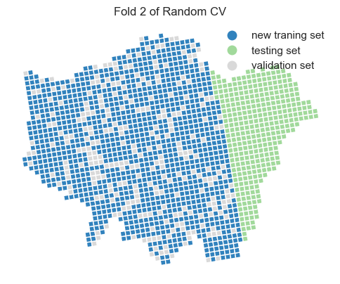
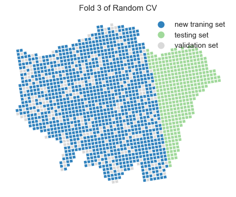
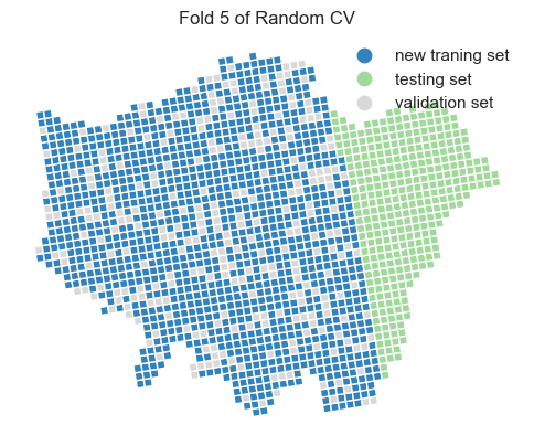
We have previously discussed spatial CV and its importance. Here, the random CV may cause data leakage issues when splitting the original traning data into a new training set (80%) and new test/validation set (20%) from the original training data. We will analyze and compare the differences of trained SVR performance between random CV and spatial CV.

# we integrate the training and validation indices into the gdf for plotting
for i in range(0, 5):
    gdf_london_grid_poi_crime[f'index_gr'] = gdf_london_grid_poi_crime.index
    gdf_london_grid_poi_crime[f'Fold {i + 1}'] = gdf_london_grid_poi_crime.index_gr.apply(
        lambda x: 'new traning set' if x in tr_idx_list[i] else (
            'validation set' if x in va_idx_list[i] else 'testing set'))

    # we plot the train and test via the index on the grids
    fig, ax = plt.subplots(1, 1, figsize=(6, 6))
    gdf_london_grid_poi_crime.plot(ax=ax, column=f'Fold {i + 1}', cmap='tab20c', legend=True, figsize=(8, 6),
                                   legend_kwds={'frameon': False})
    plt.title(f'Fold {i + 1} of Random CV')
    ax.axis('off')
    plt.show()

gdf_london_grid_poi_crime_train

	OBJECTID	grd_fixid	grd_floaid	grd_newid	pcd_count	tot_p	tot_m	tot_f	tot_hh	GlobalID	...	crime_counts	index_gr	Fold 1	Fold 2	Fold 3	Fold 4	Fold 5	centroid_x	centroid_y	cluster
0	214289	4.0.35930000.32030000	3593.3203.4	1kmN3203E3593	3	9	5	4	5	9f0c1e1f-e8fa-40ca-a969-d1aedbefa750	...	5.0	0	new traning set	new traning set	validation set	new traning set	new traning set	503482.732613	175573.691920	2
1	214290	4.0.35930000.32040000	3593.3204.4	1kmN3204E3593	54	1957	1029	928	833	e2530627-9630-4200-ae13-788341456d76	...	13.0	1	new traning set	new traning set	new traning set	new traning set	validation set	503319.399333	176558.376435	2
2	214865	4.0.35940000.32020000	3594.3202.4	1kmN3202E3594	13	445	223	222	169	bf801f98-5376-4c37-8bcb-d80ae9af1f0b	...	0.0	2	new traning set	new traning set	validation set	new traning set	new traning set	504633.969678	174752.667917	2
3	214866	4.0.35940000.32030000	3594.3203.4	1kmN3203E3594	3	34	18	16	11	472a8640-40e0-4c94-8eb5-37647847dc99	...	1519.0	3	new traning set	validation set	new traning set	new traning set	new traning set	504470.650327	175737.362096	2
4	214867	4.0.35940000.32040000	3594.3204.4	1kmN3204E3594	1	15	9	6	8	c21982c0-0d13-43df-8fa5-f77c28fba3d6	...	0.0	4	new traning set	new traning set	new traning set	validation set	new traning set	504307.315366	176722.053398	2
...	...	...	...	...	...	...	...	...	...	...	...	...	...	...	...	...	...	...	...	...	...
1381	233221	4.0.36330000.32050000	3633.3205.4	1kmN3205E3633	149	17774	9897	7877	4810	81df1f73-eabc-432a-96cf-354e3b7e1e58	...	3716.0	1381	new traning set	new traning set	validation set	new traning set	new traning set	542671.312583	184090.897282	1
1382	233222	4.0.36330000.32060000	3633.3206.4	1kmN3206E3633	138	17822	9494	8328	4784	c5616e02-895d-4669-8768-8357a13dd7f2	...	1345.0	1382	new traning set	validation set	new traning set	new traning set	new traning set	542507.875127	185075.860321	1
1383	233223	4.0.36330000.32070000	3633.3207.4	1kmN3207E3633	55	6018	3233	2785	1854	8f730656-d48d-4f99-928b-30cb304f3058	...	861.0	1383	new traning set	new traning set	new traning set	new traning set	validation set	542344.421880	186060.820314	1
1384	233224	4.0.36330000.32080000	3633.3208.4	1kmN3208E3633	19	1544	734	810	529	40f56c08-6faf-46f0-b86f-43a4633d560e	...	152.0	1384	new traning set	new traning set	new traning set	validation set	new traning set	542180.952846	187045.777269	1
1385	233225	4.0.36330000.32090000	3633.3209.4	1kmN3209E3633	68	4602	2308	2294	1387	65b9480d-a4f7-4b82-9731-65080d9b5f31	...	419.0	1385	new traning set	new traning set	validation set	new traning set	new traning set	542017.468026	188030.731192	1

1386 rows × 24 columns

# use groupcv in sklearn to select the data
from sklearn.model_selection import GroupKFold

# Define the number of splits
n_splits = 5
# Create a GroupKFold object
group_kfold = GroupKFold(n_splits=n_splits)
# Initialize an empty list to store the mean squared errors
g_mse_list = []
# Initialize an empty list to store the training and validation indices
g_tr_idx_list = []
g_va_idx_list = []
# Loop through the splits
for i, (g_train_idx, g_va_idx) in enumerate(
        group_kfold.split(X_train_scaled, y_train_scaled, groups=gdf_london_grid_poi_crime_train['cluster'])):
    X_tr, X_va = X_train_scaled[g_train_idx], X_train_scaled[g_va_idx]
    y_tr, y_va = y_train_scaled[g_train_idx], y_train_scaled[g_va_idx]
    model = svm_model.set_params(**{'C': 10, 'epsilon': 0.3, 'gamma': 0.1, 'kernel': 'poly'})
    model.fit(X_tr, y_tr.ravel())
    preds = model.predict(X_va)
    g_mse = mean_squared_error(y_va, preds)
    print(f"Fold {i + 1}: MSE = {g_mse:.2f}",
          f"Training samples length = {len(train_idx.tolist())},",
          f"Validation samples length = {len(va_idx.tolist())}")
    g_mse_list.append(g_mse)
    print('Mean of mses:', f'{np.mean(g_mse_list):.2f}')
    g_tr_idx_list.append(g_train_idx.tolist())
    g_va_idx_list.append(g_va_idx.tolist())

Fold 1: MSE = 0.31 Training samples length = 1109, Validation samples length = 277
Mean of mses: 0.31
Fold 2: MSE = 0.36 Training samples length = 1109, Validation samples length = 277
Mean of mses: 0.34
Fold 3: MSE = 0.36 Training samples length = 1109, Validation samples length = 277
Mean of mses: 0.35
Fold 4: MSE = 0.76 Training samples length = 1109, Validation samples length = 277
Mean of mses: 0.45
Fold 5: MSE = 0.24 Training samples length = 1109, Validation samples length = 277
Mean of mses: 0.41

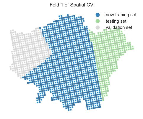
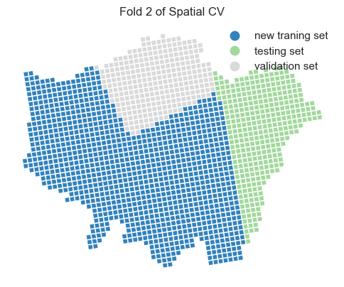
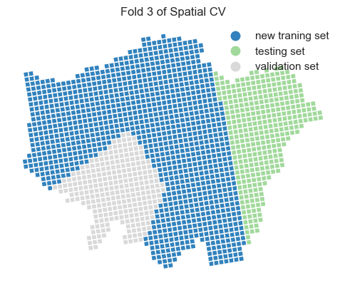
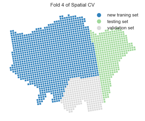
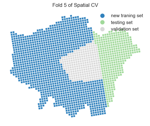
# We integrate the training and validation indices into the gdf for plotting
for i in range(0, 5):
    gdf_london_grid_poi_crime[f'index_gr'] = gdf_london_grid_poi_crime.index
    gdf_london_grid_poi_crime[f'Group Fold {i + 1}'] = gdf_london_grid_poi_crime.index_gr.apply(
        lambda x: 'new traning set' if x in g_tr_idx_list[i] else (
            'validation set' if x in g_va_idx_list[i] else 'testing set'))
    # we plot the train and test via the index on the grids
    fig, ax = plt.subplots(1, 1, figsize=(6, 6))
    gdf_london_grid_poi_crime.plot(ax=ax, column=f'Group Fold {i + 1}', cmap='tab20c', legend=True, figsize=(8, 6),
                                   legend_kwds={'frameon': False})
    plt.title(f'Fold {i + 1} of Spatial CV')
    ax.axis('off')
    plt.show()

Two important parameter settings in grid_search.fit() and GridSearchCV():

• cv: this should be defined as the group_kfold from the GroupKFold

• groups: this should be defined as the array/list groups_label from the training set

Hyperparameter via GridSearch and Spatial CV

Training set performance metrics

Testing set performance metrics

We observe that the model’s performance decreases when using spatial cross-validation and grid search compared to the random cross-validation approach. Additionally, the optimal hyperparameters have changed. This suggests that, in the context of spatial prediction, the current model is more robust than the one we previously trained, even though its overall performance appears to be lower.