Week1 Lab Tutorial Timeline

Time	Activity
16:00–16:05	Introduction — Overview of the main tasks for the lab tutorials
16:05–16:45	Tutorial: Conda Setup — Follow Section 0 of the Jupyter Notebook to set up Conda and configure the geospatial analytics environment
16:45–17:30	Tutorial: Geospatial Data Types — Follow Section 1 of the Jupyter Notebook to learn about geospatial data types
17:30–17:55	Quiz — Complete quiz tasks
17:55–18:00	Wrap-up — Recap key points and address final questions

For this module’s lab tutorials, you can download all the required data using the provided link (click).

Please make sure that both the Jupyter Notebook file and the data and img folder are placed in the same directory (specifically within the STBDA_lab folder) to ensure the code runs correctly.

Week 1 Key Takeaways:

• install conda (e.g., Anaconda) and use the conda commands to configure the environment;

• understand the geospatial data formats and geometric objects types;

• use the Geopandas to do the geospatial data reading and saving, projection, and processing in Jupyter-Lab.

0 Set up conda and configuration

What is conda and why do we need it ?

Conda is an environment management system that helps users to easily install, manage, and switch between different environments and dependencies. In geo big data analytics, as conflicts between libraries or packages can occasionally occur resulting in errors, conda allows you to set up multiple isolated environments on your computer, each with different versions of Python and various libraries (e.g., geopandas).

0.1 Install conda

There are two options for using the conda installer: Anaconda and Miniconda.

(This workshop introduces installing Anaconda which is beginner-friendly, then provides instruction links for installing Miniconda.)

• Anaconda is an open-source platform for data science and AI by offering Python, conda, and tremendous pre-installed packages (e.g., NumPy, Pandas, Jupyter). It also includes Anaconda Navigator, a GUI for managing environments and tools. Large size around 3G.

• Miniconda is a smaller version of Anaconda, including only conda, Python, and essential dependencies. Users can install packages as needed, providing more flexibility and control. GUI is not included (command-line only). Small size around 100M.

Step 1: Visit the Anaconda download page (click) and select the installer compatible with your operating system (e.g., Windows, macOS, or Linux).

Step 2: Run the installer and complete the installation.

For Windows:

1. Make sure that you have downloaded the Anaconda3 installer with 3.x python version, e.g., Anaconda3-2024.10-1-Windows-x86_64.exe;

2. Locate the downloaded .exe file and double-click to start installation;

3. License agreement: Click I Agree;

4. Installation type: Choose Just Me (recommended for single-user setups);

5. Destination folder: Keep the default path (e.g., C:\Users<YourUsername>\Anaconda3);

6. Click Install and wait for completion.

For macOS:

1. Make sure that you haved the downloaded .pkg file (e.g., Anaconda3-2024.10-1-MacOSX-arm64.pkg for Apple silicon and Anaconda3-2024.10-1-MacOSX-x86_64.pkg for Intel chip);

2. Introduction: Click Continue –> License Agreement: Click Agree;

3. Choose Install for me only (recommended);

4. Destination: Select your hard drive (default);

5. Click Install and wait for completion.

For Linux:

1. Select Linux and download the .sh file (e.g., Anaconda3-2024.10-1-Linux-x86_64.sh);

2. Open Terminal and navigate to the download folder by using linux bash commands:

   cd ~/Downloads
   

3. Run the installer in teriminal:

    bash Anaconda3-2024.10-1-Linux-x86_64.sh 
   

4. License Agreement: Press Enter to scroll, then type yes to accept;

5. Installation Location: Keep the default path (e.g., ~/anaconda3) or customize;

6. Initialize Conda: Type yes to add Anaconda to your PATH in ~/.bashrc (recommended).

Step 3: Verify Anaconda installation

For Windows:

Launch Anaconda Navigator (from the Start Menu) to confirm the base environment are ready.

or open Anaconda Prompt in Anaconda Navigator, there is a (base) ahead of the commnad line ((base) C:\Users\username>) as conda automatically activates the (base) environment in the Anaconda Prompt. Then check the conda version by typing following commands and enter

conda --version

or

conda -V

For macOS:

Open the terminal, you can find (base) hostname:~ username$ and type conda –version to check the version.

For Linux:

Open the terminal, you can find (base) username@hostname:~$ and type conda –version to check the version.

Installing Minicoda

• Option 1: You can download the Miniconda installer for different operating systems from this page and follow the same installation process as we previously introduced for Anaconda.

• Option 2: You can download Miniconda using the command line in the terminal to install it. Instructions for different operating systems can be found on this page.

0.2 Managing conda

0.2.1 Creating environment

Open the Anaconda Prompt in the Anaconda Navigator, then create an environment named STBDA-test using the following commands:

conda create --name STBDA-test

When conda asks you to proceed, type y and enter. This creates the STBDA-test environment in ananaconda3/envs/.

0.2.2 Activate environment

To activate environemnt STBDA-test, typing:

conda activate STBDA-test

There is a (STBDA-test) ahead of the commnad line right now which means the environment STBDA-testhas neen activated.

0.2.3 Installing python libraries/tools

We can now install the required libraries/tools in the STBDA-test environment, such as pandas:

conda install pandas

or

conda install -c conda-forge pandas

or

pip install pandas

0.2.4 Use a YAML (.yml) file in conda for environment management

A .yml file defines the environment’s name, channels, and dependencies, which can help you to replicate the entire environment on another computer/device when needed.

In this module, we will use STBDA.yml to set up a conda environment named STBDA for all the practical exercises.

If you are using conda in macOS, you can download the STBDA.yml at here (click).

If you are using conda in windows, please download the YAML STBDA_win.yml at here (click).

You need to put the STBDA.yml in your current working directory (the directory you’re in when you run the command).

Check the current working directory in anaconda_prompt of Windows:

cd

For macOS/Linux terminal:

pwd

Now, put the STBDA.yml to the current working path folder, then deactivate the STBDA-test enviroment by inputting conda deactivate, and create a STBDA env from the yml by:

conda env create -f STBDA.yml

or in the win version:

conda env create -f STBDA_win.yml

Option: In above command, you can replace STBDA.yml to the absolute/full path. e.g., /path/to/your/STBDA.yml (in Windows, right click to the file and select Copy as path).

Once all prerequisite libraries are installed, use conda activate STBDA to activate the environment and then run jupyter-lab to start Jupyter Lab.

0.2.5 Other conda commands

Check/verify all installed environment:

conda env list

Rename environment:

conda rename --name oldname newname

Remove environment:

conda rename --name envname  --all

Notice: You can check other useful Conda commands to help you configure environment management on this webpage.

1 Geospatial data types

In this module, we will introduce the fundamental geospatial data types and processing techniques with GeoPandas, which is a Python library for working with geospatial data. It extends the capabilities of Pandas to handle spatial data for users to perform geospatial operations and analyses easily.

# Import required libraries
import pandas as pd
import geopandas  as gpd

Geopandas dataframe (GeoDataFrame) contains three parts:

• index: The index column is a unique identifier for each row in the GeoDataFrame. It can be a simple integer index or a more complex index based on the data.

• data: The data columns contain the attribute information associated with each geometric feature. These columns can include various data types, such as integers, floats, strings, and dates.

• geometry: The geometry column contains the geometric representation of the features (e.g., points, lines, polygons). It is a special column that stores geometric objects using Shapely library.

Geospatial data types:

• Vector data: Represents geographic features using points, lines, and polygons (geometry types). Each feature has associated attributes stored in a table. Common file formats include Shapefile, GeoJSON, and KML (In this module, we mainly focus on this type of geospatial data type).

Feature	Shapefile	GeoJSON	KML
Format Type	Binary (requires multiple files)	Text (JSON-based, lightweight)	Text (XML-based, heavier)
Main Usage	Professional GIS software	Web mapping and APIs (e.g., Leaflet, Mapbox)	Google Earth, simple visualization
File Size & Efficiency	Efficient but needs .shp, .shx, .dbf files together	Light, easy to transfer over web	Larger files, less ideal for large datasets

Big data format:

Feature	Parquet / GeoParquet	GeoPackage (.gpkg)	GeoJSONSeq / JSONL
Format Type	Binary (columnar, optimized for analytics)	Binary (SQLite-based single-file database)	Text-based (line-delimited GeoJSON)
Main Usage	Big data processing, cloud analytics, fast I/O	Desktop GIS, mobile apps, portable multi-layer data	Streaming spatial data, logging, web pipelines
File Size & Efficiency	Very compact, highly efficient for large/tabular data	Compact, self-contained but larger than Parquet	Lightweight per line, but not efficient at scale
Multi-layer Support	1 table per file, but easily batched	Fully supports multiple vector and raster layers	No layer structure

• Raster data: Represents geographic information as a grid of pixels, where each pixel has a value representing a specific attribute (e.g., elevation, temperature). Common formats include GeoTIFF and NetCDF.

1.1 Fundamental geometric objects

Geometry types / geometric objects:

• Points: Represent discrete locations (e.g., cities, landmarks).

  • MultiPoint: A collection of multiple points, often used to represent clusters of discrete locations (e.g., a group of cities).

• LineString: Represent linear features (e.g., roads, rivers).

  • MultiLineString: A collection of multiple lines, often used to represent complex linear features (e.g., a river with multiple branches).

• Polygons: Represent areas (e.g., countries, lakes).

  • MultiPolygon: A collection of multiple polygons, often used to represent complex areas (e.g., a country with multiple islands).

We use a python library called Shapely to handle nad process the geometric objects. We don’t need to install it separately as it is already included in the GeoPandas library.

# Import the required libraries
from shapely.geometry import Point, LineString, Polygon, MultiPoint, MultiLineString, MultiPolygon

1.1.1 Point

# Create a point object
point1 = Point(1, 2)
point2 = Point(3, 4)

# The point object
point1

# Print the point objects type in python
type(point1)

shapely.geometry.point.Point

# Or we can use the geom_type to check the type of the point object
point1.geom_type

'Point'

Point attributes

# We can also check the coordinate info (x, y) of the point object
print(list(point1.coords), point1.x, point1.y)

[(1.0, 2.0)] 1.0 2.0

Distance between two points

While the distance between two points is calculated using the Euclidean distance formula, which is the straight-line distance between two points in a Cartesian coordinate system (we will introduce the coordinate reference system (CRS) later). In other words, checking measurement unit (meter, feet or mile) in the CRS you’re using is important.

# Calculate the distance between two points
point1.distance(point2)

2.8284271247461903

Creating a GeoDataframe with df

# Create a GeoDataFrame with point1 and point2
# Create a DataFrame with point1 and point2
df = pd.DataFrame({'name': ['pt1', 'pt2'], 'geometry': [point1, point2]})
# Create a GeoDataFrame from the DataFrame
gdf1 = gpd.GeoDataFrame(df, geometry='geometry')
gdf1

	name	geometry
0	pt1	POINT (1 2)
1	pt2	POINT (3 4)

If there is a large set of coords in a file, we can use gpd.points_from_xy() to create a GeoDataFrame with points from the x and y coordinates.

# Create a DataFrame with x and y coordinates
df = pd.DataFrame({'x': [1, 2, 3, 6], 'y': [4, 5, 6, 8]})
# Create a GeoDataFrame from the DataFrame
gdf2 = gpd.GeoDataFrame(df, geometry=gpd.points_from_xy(df.x, df.y))
gdf2

	x	y	geometry
0	1	4	POINT (1 4)
1	2	5	POINT (2 5)
2	3	6	POINT (3 6)
3	6	8	POINT (6 8)

1.1.2 LineString

# Create a LineString object
line1 = LineString([(0, 0), (1, 1), ]) # A line is made of two points
line2 = LineString([(0, 0), (1, 2), (2, 2)]) # A line is made of three points
line3 = LineString([(0, 0), (0, 2), (2, 3), (3, 1)]) # A line with four points

# The LineString object
line1

# The LineString object
line2

# The LineString object
line3

# Print the LineString objects type in python
type(line1)

shapely.geometry.linestring.LineString

# Or we can use the geom_type to check the type of the LineString object
line1.geom_type

'LineString'

LineString attributes

# We can also check the coordinate info (x, y) of points within the LineString object
print('line1', list(line1.coords), line1.xy)
print('line2', list(line2.coords), line2.xy)
print('line3', list(line3.coords), line3.xy)

line1 [(0.0, 0.0), (1.0, 1.0)] (array('d', [0.0, 1.0]), array('d', [0.0, 1.0]))
line2 [(0.0, 0.0), (1.0, 2.0), (2.0, 2.0)] (array('d', [0.0, 1.0, 2.0]), array('d', [0.0, 2.0, 2.0]))
line3 [(0.0, 0.0), (0.0, 2.0), (2.0, 3.0), (3.0, 1.0)] (array('d', [0.0, 0.0, 2.0, 3.0]), array('d', [0.0, 2.0, 3.0, 1.0]))

Calculate the length of the LineString object

# Calculate the length of the LineString object
line1.length, line2.length, line3.length

(1.4142135623730951, 3.23606797749979, 6.47213595499958)

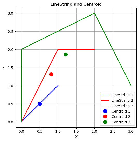
The centroid of a LineString

The centroid of a LineString is the point that represents the geometric center of the line. It is calculated as the average of the coordinates of all points in the LineString. The centroid is not necessarily a point on the line itself, but it is the point that minimizes the distance to all points on the line.

# Calculate the centroid of the LineString object
line1.centroid, line2.centroid, line3.centroid

(<POINT (0.5 0.5)>, <POINT (0.809 1.309)>, <POINT (1.209 1.864)>)

# we use matplotlib to plot the LineStrings and their centroids

import matplotlib.pyplot as plt
# Create a figure and axis
fig, ax = plt.subplots(figsize=(6, 6))
# Plot the LineString object
x, y = line1.xy
ax.plot(x, y, color='blue', linewidth=2, label='LineString 1')
x, y = line2.xy
ax.plot(x, y, color='red', linewidth=2, label='LineString 2')
x, y = line3.xy
ax.plot(x, y, color='green', linewidth=2, label='LineString 3')
# Plot the centroid of the LineString object
ax.plot(line1.centroid.x, line1.centroid.y, 'o', color='blue', markersize=10, label='Centroid 1')
ax.plot(line2.centroid.x, line2.centroid.y, 'o', color='red', markersize=10, label='Centroid 2')
ax.plot(line3.centroid.x, line3.centroid.y, 'o', color='green', markersize=10, label='Centroid 3')
ax.grid()
# Add a title and labels
ax.set_title('LineString and Centroid')
ax.set_xlabel('X')
ax.set_ylabel('Y')
# Add a legend
ax.legend()
# Show the plot
plt.show()

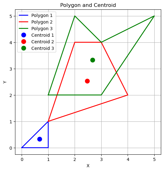
1.1.3 Polygon

Building a polygon is not as simple as a point or a line. A polygon is made of multiple points, and the first and last points must be the same to close the polygon. The points are connected in the order they are defined, forming the edges of the polygon.

# Create a Polygon object
polygon1 = Polygon([(0, 0), (1, 1), (1, 0), (0, 0)]) # A polygon is made of three points
polygon2 = Polygon([(1, 1), (2, 4), (3, 4), (4, 2), (1, 1)]) # A polygon is made of four points
polygon3 = Polygon([(1, 2), (2, 5), (3, 4),(5, 5), (3, 2), (1, 2)]) # A polygon is made of five points

# The Polygon object
polygon1

# The Polygon object
polygon2

# The Polygon object
polygon3

# we can also create a polygon using the LineString object, the polygon is made of four points, it will be closed automatically.
polygon4 = Polygon(line3)

# The Polygon object
polygon4

# we can also create a polygon with a hole using sell and hole
# The outer boundary of the polygon
# The inner boundary of the polygon (the hole)
outer_boundary = [(0, 0), (4, 0), (4, 4), (0, 4), (0, 0)]
inner_boundary = [(1, 1), (1, 3), (3, 3), (3, 1), (1, 1)]
polygon5 = Polygon(shell=outer_boundary, holes=[inner_boundary])

# The Polygon object
polygon5

# Print the Polygon objects type in python
type(polygon1)

shapely.geometry.polygon.Polygon

# Or we can use the geom_type to check the type of the Polygon object
polygon1.geom_type

'Polygon'

Polygon attributes

# We can also check the coordinate info (x, y) of points within the Polygon object
print('polygon2', list(polygon2.exterior.coords), polygon2.exterior.xy)

polygon2 [(1.0, 1.0), (2.0, 4.0), (3.0, 4.0), (4.0, 2.0), (1.0, 1.0)] (array('d', [1.0, 2.0, 3.0, 4.0, 1.0]), array('d', [1.0, 4.0, 4.0, 2.0, 1.0]))

# get the exterior and interior coordinates of the polygon5
print('polygon5', list(polygon5.exterior.coords), polygon5.exterior.xy)
print('polygon5', list(polygon5.interiors[0].coords), polygon5.interiors[0].xy)

polygon5 [(0.0, 0.0), (4.0, 0.0), (4.0, 4.0), (0.0, 4.0), (0.0, 0.0)] (array('d', [0.0, 4.0, 4.0, 0.0, 0.0]), array('d', [0.0, 0.0, 4.0, 4.0, 0.0]))
polygon5 [(1.0, 1.0), (1.0, 3.0), (3.0, 3.0), (3.0, 1.0), (1.0, 1.0)] (array('d', [1.0, 1.0, 3.0, 3.0, 1.0]), array('d', [1.0, 3.0, 3.0, 1.0, 1.0]))

# The exterior length of the polygon
print('polygon2', polygon2.exterior.length)

polygon2 9.56062329783655

# The exterior and interior length of the polygon5
print('polygon5', polygon5.exterior.length, polygon5.interiors[0].length)

polygon5 16.0 8.0

# Calculate the area of the Polygon object
polygon1.area, polygon2.area, polygon3.area, polygon4.area, polygon5.area

(0.5, 5.0, 6.0, 5.5, 12.0)

# we use matplotlib to plot the Polygons and their centroids
# Create a figure and axis
fig, ax = plt.subplots(figsize=(6, 6))
# Plot the Polygon object
x, y = polygon1.exterior.xy
ax.plot(x, y, color='blue', linewidth=2, label='Polygon 1')
x, y = polygon2.exterior.xy
ax.plot(x, y, color='red', linewidth=2, label='Polygon 2')
x, y = polygon3.exterior.xy
ax.plot(x, y, color='green', linewidth=2, label='Polygon 3')
# Plot the centroid of the Polygon object
ax.plot(polygon1.centroid.x, polygon1.centroid.y, 'o', color='blue', markersize=10, label='Centroid 1')
ax.plot(polygon2.centroid.x, polygon2.centroid.y, 'o', color='red', markersize=10, label='Centroid 2')
ax.plot(polygon3.centroid.x, polygon3.centroid.y, 'o', color='green', markersize=10, label='Centroid 3')
ax.grid()
# Add a title and labels
ax.set_title('Polygon and Centroid')
ax.set_xlabel('X')
ax.set_ylabel('Y')
# Add a legend
ax.legend()
# Show the plot
plt.show()

1.1.4 MultiPoint, MultiLineString, and MultiPolygon

# Create a MultiPoint object
multipoint = MultiPoint([point1, point2])

# The MultiPoint object
multipoint

# Print the MultiPoint objects type in python
type(multipoint)

shapely.geometry.multipoint.MultiPoint

# Or we can use the geom_type to check the type of the MultiPoint object
multipoint.geom_type

'MultiPoint'

# Create a MultiLineString object
multiline = MultiLineString([line1, line2, line3])

# The MultiLineString object
multiline

# Print the MultiLineString objects type in python
type(multiline)

shapely.geometry.multilinestring.MultiLineString

# Or we can use the geom_type to check the type of the MultiLineString object
multiline.geom_type

'MultiLineString'

# Create a MultiPolygon object
multipolygon = MultiPolygon([polygon1, polygon2, polygon3])

# The MultiPolygon object
multipolygon

# Print the MultiPolygon objects type in python
type(multipolygon)

shapely.geometry.multipolygon.MultiPolygon

# Or we can use the geom_type to check the type of the MultiPolygon object
multipolygon.geom_type

'MultiPolygon'

Noted: we can also get the length, area, centroid, and distance of the MultiPoint, MultiLineString, and MultiPolygon objects.

1.2 Map Projection

Coordinate reference system

A Coordinate Reference System (CRS) defines how the Earth’s curved surface is represented on a flat map using coordinates. It specifies both the shape of the Earth (through a datum) and the method of projecting that shape onto a two-dimensional plane. Without a CRS, spatial data cannot be accurately positioned, nor can it be reliably combined with other datasets.

CRS Name	EPSG Code	Type	Notes
OSGB36 / British National Grid	EPSG:27700	Projected	The main CRS for mapping in Great Britain. Uses a Transverse Mercator projection and the OSGB36 datum.
WGS 84	EPSG:4326	Geographic	Used globally (e.g. GPS systems, Google Maps). Coordinates in latitude and longitude.
Irish Grid (Ireland and Northern Ireland)	EPSG:29902	Projected	Separate grid for Ireland (but related principles).
Web Mercator	EPSG:3857	Projected	Used by many web mapping applications (e.g. Google Maps, OpenStreetMap). Distorts areas and distances, but preserves angles.
NAD83 / UTM Zone 10N	EPSG:26910	Projected	Used in North America. Based on the UTM system, which divides the world into a series of zones.

EPSG (European Petroleum Survey Group) codes are a standardized set of identifiers for coordinate reference systems. They provide a unique identifier for each CRS, making it easier to reference and use them in GIS applications.

You can check all reference systems in the EPSG registry here (click).

Geographic vs. Projected Coordinate Systems

Type	Geographic Coordinate System (GCS)	Projected Coordinate System (PCS)
Coordinates	Latitude (Y) and Longitude (X), in degrees	X and Y values in meters, feet, or other linear units
Surface	Curved (earth-like, 3D ellipsoid)	Flat (2D map surface)
Examples	WGS84 (EPSG:4326), NAD83 (EPSG:4269)	UTM, State Plane, British National Grid
Good for	Global data, navigation, GPS	Local maps, accurate distances, areas, engineering
Issues	Hard to measure real distances (degrees aren’t equal in size everywhere)	Distortions (shape, area, distance, direction) — you have to choose which to minimize

Now, we use the UK Countries Boundaries data downloaded from ONS Open Geography portal as an example with GeoPandas.

# Load the shapefile, please note the .shp file is a part of the shapefile, and you need to download all the files in the same folder.
gdf_uk_1 = gpd.read_file("data/Countries_December_2024_Boundaries_UK/CTRY_DEC_2024_UK_BFC.shp")

# We get the geo-dataframe gdf_uk_1, which contains the geometry column (which is a multipolygon) and other attribute columns (four rows refer to four countries).
gdf_uk_1

	CTRY24CD	CTRY24NM	CTRY24NMW	BNG_E	BNG_N	LONG	LAT	GlobalID	geometry
0	E92000001	England	Lloegr	394883	370883	-2.07812	53.2350	5cad1ec2-bbe1-4ec4-bcd9-ba0cb9c3fc1f	MULTIPOLYGON (((83962.84 5401.15, 83970.68 540...
1	N92000002	Northern Ireland	Gogledd Iwerddon	86544	535337	-6.85571	54.6150	8d8effb1-0159-4cd6-b856-21a8754b4693	MULTIPOLYGON (((131198.094 468427.673, 131196....
2	S92000003	Scotland	Yr Alban	277744	700060	-3.97094	56.1774	a158e058-71b1-4272-b4bf-91c241d13159	MULTIPOLYGON (((265944.63 543512.72, 265945.83...
3	W92000004	Wales	Cymru	263405	242881	-3.99418	52.0674	c78b0dcc-7d89-42b2-9667-57aa91a55e74	MULTIPOLYGON (((322081.699 165165.901, 322082....

# Geoseries is a class of geo-df that stores geometric representations using Shapely library.
type(gdf_uk_1.geometry)

geopandas.geoseries.GeoSeries

# the geometry column contains the geometric representation of the features (e.g., points, lines, polygons).
type(gdf_uk_1.geometry[0])

shapely.geometry.multipolygon.MultiPolygon

# Load the geojson file; you may observe that the geojson file is much smaller than the shapefile.
gdf_uk_2 = gpd.read_file("data/Countries_December_2024_Boundaries_UK.geojson")

# We get the geo-dataframe gdf_uk_2, which contains the same information as the gdf_uk_1 from shp.
# However, the values in the geometry column are different, but they represent the same multipolygon geometries.
gdf_uk_2

	FID	CTRY24CD	CTRY24NM	CTRY24NMW	BNG_E	BNG_N	LONG	LAT	GlobalID	geometry
0	1	E92000001	England	Lloegr	394883	370883	-2.07812	53.23497	bd411920-e7ea-4f71-b6c8-5f1d24ec92d3	MULTIPOLYGON (((-6.34905 49.89822, -6.32842 49...
1	2	N92000002	Northern Ireland	Gogledd Iwerddon	86544	535337	-6.85571	54.61502	652c0c4b-647b-4565-b9ed-e9c17ec5834c	MULTIPOLYGON (((-5.52389 54.67041, -5.52451 54...
2	3	S92000003	Scotland	Yr Alban	277744	700060	-3.97094	56.17744	97bb1057-3e8d-4ad8-83ef-4577d1bb4d9c	MULTIPOLYGON (((-3.06033 54.98452, -3.06337 54...
3	4	W92000004	Wales	Cymru	263405	242881	-3.99418	52.06742	f7c86b8c-b705-44b7-bb7b-46323f7bddfe	MULTIPOLYGON (((-4.30971 51.56253, -4.31141 51...

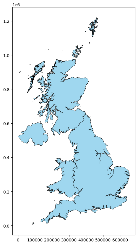
# Check the CRS of the gdf_uk_1
gdf_uk_1.crs

<Projected CRS: EPSG:27700>
Name: OSGB36 / British National Grid
Axis Info [cartesian]:
- E[east]: Easting (metre)
- N[north]: Northing (metre)
Area of Use:
- name: United Kingdom (UK) - offshore to boundary of UKCS within 49°45'N to 61°N and 9°W to 2°E; onshore Great Britain (England, Wales and Scotland). Isle of Man onshore.
- bounds: (-9.01, 49.75, 2.01, 61.01)
Coordinate Operation:
- name: British National Grid
- method: Transverse Mercator
Datum: Ordnance Survey of Great Britain 1936
- Ellipsoid: Airy 1830
- Prime Meridian: Greenwich

# we can also plot the gdf_uk_1 check the projection: x and y are in metre.
gdf_uk_1.plot(color="skyblue", edgecolor="black", lw= 0.5, alpha=0.8, figsize=(10, 10))

<Axes: >

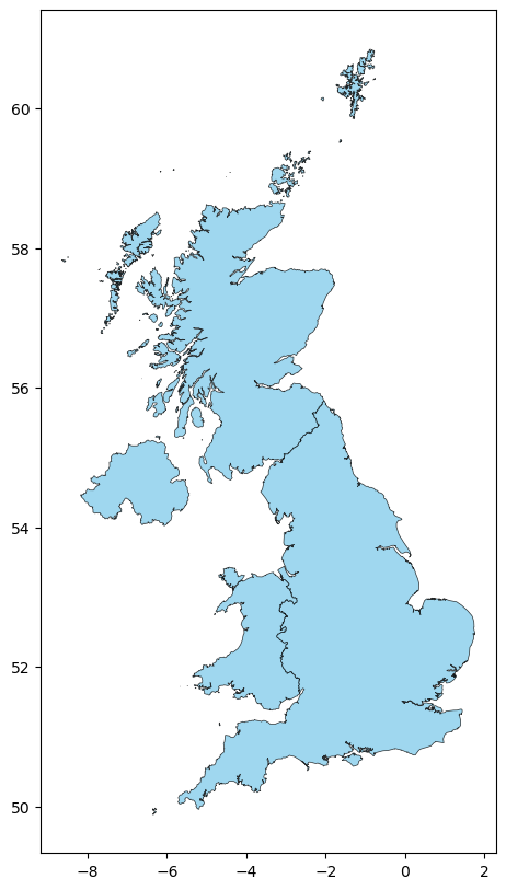
# Check the CRS of the gdf_uk_2
gdf_uk_2.crs

<Geographic 2D CRS: EPSG:4326>
Name: WGS 84
Axis Info [ellipsoidal]:
- Lat[north]: Geodetic latitude (degree)
- Lon[east]: Geodetic longitude (degree)
Area of Use:
- name: World.
- bounds: (-180.0, -90.0, 180.0, 90.0)
Datum: World Geodetic System 1984 ensemble
- Ellipsoid: WGS 84
- Prime Meridian: Greenwich

# we can also plot the gdf_uk_2 check the projection: x and y are in degree.
gdf_uk_2.plot(color="skyblue", edgecolor="black", lw= 0.5, alpha=0.8, figsize=(10, 10))

<Axes: >

What is a map projection for coordinates:

A projection is a mathematical transformation that converts 3D geographic coordinates (latitude and longitude) into 2D Cartesian coordinates (X, Y).

# we can use geopandas to implement the projection of the gdf_uk_2, i.e., we can change the CRS of the gdf_uk_2 to the same as the gdf_uk_1.
gdf_uk_2 = gdf_uk_2.to_crs(epsg="27700")

# The coordinate information in the geometry column of gdf_uk_2 has been changed from degree to meter, i.e., the same as the gdf_uk_1.
gdf_uk_2

	FID	CTRY24CD	CTRY24NM	CTRY24NMW	BNG_E	BNG_N	LONG	LAT	GlobalID	geometry
0	1	E92000001	England	Lloegr	394883	370883	-2.07812	53.23497	bd411920-e7ea-4f71-b6c8-5f1d24ec92d3	MULTIPOLYGON (((87801.366 8851.285, 89245.07 8...
1	2	N92000002	Northern Ireland	Gogledd Iwerddon	86544	535337	-6.85571	54.61502	652c0c4b-647b-4565-b9ed-e9c17ec5834c	MULTIPOLYGON (((172874.784 536295.76, 172826.7...
2	3	S92000003	Scotland	Yr Alban	277744	700060	-3.97094	56.17744	97bb1057-3e8d-4ad8-83ef-4577d1bb4d9c	MULTIPOLYGON (((332243.529 566060.503, 332047....
3	4	W92000004	Wales	Cymru	263405	242881	-3.99418	52.06742	f7c86b8c-b705-44b7-bb7b-46323f7bddfe	MULTIPOLYGON (((240000.014 187378.451, 239878....

# we can also plot the gdf_uk_2 check the projection: x and y are transferred to metre.
gdf_uk_2.plot(color="skyblue", edgecolor="black", lw= 0.5, alpha=0.8, figsize=(10, 10))
plt.xlim(0.)
plt.ylim(0.)
# let y ticks show all the numbers
plt.ticklabel_format(style='plain', axis='y')

Week1 Quiz

• Q1. Load the geojson file of local authority district boundaries in the UK named ‘Local_Authority_Districts_December_2024_Boundaries_UK_BSC.geojson’ in the data folder and check the columns: How many local authorities in the UK? How many types of geometry in the geometry column?

• Q2. Check the CRS of the loaded GeoDataframe.

• Q3. Select the ‘Kingston upon Hull, City of’ (stored in the LAD24NM column) and plotting/mapping, what is the ID (in LAD24CD) of the ‘Kingston upon Hull, City of’?

• Q4. Transfer the geometry column to the OSGB36 / British National Grid CRS (Projection) then plotting and compare the two maps.

• Q5. Save the ‘Kingston upon Hull, City of’ boundary as ‘Kingston_upon_Hull_boundary.geojson’ with WGS84 CRS in the data folder (using the gdf.to_file (driver=”GeoJSON”) function in Geopandas).

• Q6. Save the ‘Kingston upon Hull, City of’ boundary as ‘Kingston_upon_Hull_boundary.shp’ with OSGB36 / British National Grid CRS in the data folder (using the gdf.to_file (driver=”ESRI Shapefile”) function in Geopandas), then check the sizes and numbers of files in the data folder.

Q1 solution:

# Load the geojson file which is the local authority district boundaries in the UK.
gdf_uk_la = gpd.read_file("data/Local_Authority_Districts_December_2024_Boundaries_UK_BSC.geojson")

# Check the info of the gdf_uk_la, we can see the geometry column including a multipolygon and polygon.
# The gdf_uk_la contains 361 rows that mean 361 local authority districts in the UK.
gdf_uk_la

	FID	LAD24CD	LAD24NM	LAD24NMW	BNG_E	BNG_N	LONG	LAT	GlobalID	geometry
0	1	E06000001	Hartlepool		447161	531473	-1.27017	54.67613	fcc85d99-da7a-440c-aa80-b6e2a5353efe	POLYGON ((-1.25856 54.72606, -1.25186 54.71962...
1	2	E06000002	Middlesbrough		451141	516887	-1.21100	54.54468	0d2753c9-b44b-44e2-9b20-f70fd8a63e1a	POLYGON ((-1.21571 54.58107, -1.21978 54.57888...
2	3	E06000003	Redcar and Cleveland		464330	519596	-1.00657	54.56752	91793ade-9ca5-46dc-8591-7bd7fb61b233	POLYGON ((-1.11881 54.62886, -1.08462 54.6204,...
3	4	E06000004	Stockton-on-Tees		444940	518179	-1.30665	54.55688	ae16dbb0-8ebe-49c6-bff9-f3479669fd4f	POLYGON ((-1.29859 54.63116, -1.2962 54.62803,...
4	5	E06000005	Darlington		428029	515648	-1.56836	54.53534	f21d0ade-ae2f-4bff-9d85-1048cd649b5f	POLYGON ((-1.64163 54.61937, -1.63324 54.61613...
...	...	...	...	...	...	...	...	...	...	...
356	357	W06000020	Torfaen	Torfaen	327459	200480	-3.05102	51.69836	fbea0d49-4967-427d-864d-a16865da337d	POLYGON ((-3.03389 51.72551, -3.02542 51.71813...
357	358	W06000021	Monmouthshire	Sir Fynwy	337812	209231	-2.90281	51.77828	9001089d-f105-486d-ad44-451963382a2e	POLYGON ((-3.06738 51.98314, -3.03955 51.96642...
358	359	W06000022	Newport	Casnewydd	337897	187432	-2.89769	51.58231	0efd1d55-841d-4802-a798-a15d610dac80	POLYGON ((-2.8285 51.64282, -2.80568 51.62372,...
359	360	W06000023	Powys	Powys	302329	273254	-3.43532	52.34864	f0629672-87a0-4abb-b57b-698a85f634ea	POLYGON ((-3.15484 52.89809, -3.1475 52.89017,...
360	361	W06000024	Merthyr Tydfil	Merthyr Tudful	305916	206404	-3.36425	51.74841	69980e06-36dc-4e63-96c1-a4996733f28b	POLYGON ((-3.4062 51.82116, -3.40231 51.8142, ...

361 rows × 10 columns

Q2 solution:

# Check the CRS of the gdf_uk_la
gdf_uk_la.crs

<Geographic 2D CRS: EPSG:4326>
Name: WGS 84
Axis Info [ellipsoidal]:
- Lat[north]: Geodetic latitude (degree)
- Lon[east]: Geodetic longitude (degree)
Area of Use:
- name: World.
- bounds: (-180.0, -90.0, 180.0, 90.0)
Datum: World Geodetic System 1984 ensemble
- Ellipsoid: WGS 84
- Prime Meridian: Greenwich

Q3 solution:

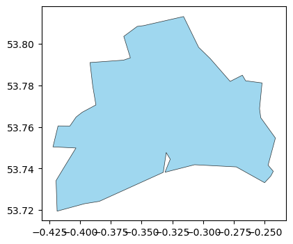
# Select the 'Kingston upon Hull, City of' (stored in the LAD24NM column) and plotting/mapping.
gdf_uk_la[gdf_uk_la["LAD24NM"] == "Kingston upon Hull, City of"].plot(color="skyblue", edgecolor="black", lw= 0.5, alpha=0.8, figsize=(6, 4))

<Axes: >

Q4 solution:

# Transfer the geometry column to the EPSG:27700 CRS (Projection) then plotting and compare the two maps.
gdf_uk_la_2 = gdf_uk_la.to_crs(epsg="27700")

# The coordinate information in the geometry column of gdf_uk_la_2 has been changed from degree to meter
gdf_uk_la_2

	FID	LAD24CD	LAD24NM	LAD24NMW	BNG_E	BNG_N	LONG	LAT	GlobalID	geometry
0	1	E06000001	Hartlepool		447161	531473	-1.27017	54.67613	fcc85d99-da7a-440c-aa80-b6e2a5353efe	POLYGON ((447851.213 537036.01, 448290.115 536...
1	2	E06000002	Middlesbrough		451141	516887	-1.21100	54.54468	0d2753c9-b44b-44e2-9b20-f70fd8a63e1a	POLYGON ((450791.114 520932.509, 450530.512 52...
2	3	E06000003	Redcar and Cleveland		464330	519596	-1.00657	54.56752	91793ade-9ca5-46dc-8591-7bd7fb61b233	POLYGON ((456987.212 526324.904, 459206.816 52...
3	4	E06000004	Stockton-on-Tees		444940	518179	-1.30665	54.55688	ae16dbb0-8ebe-49c6-bff9-f3479669fd4f	POLYGON ((445378.413 526449.708, 445536.511 52...
4	5	E06000005	Darlington		428029	515648	-1.56836	54.53534	f21d0ade-ae2f-4bff-9d85-1048cd649b5f	POLYGON ((423240.211 524970.902, 423783.816 52...
...	...	...	...	...	...	...	...	...	...	...
356	357	W06000020	Torfaen	Torfaen	327459	200480	-3.05102	51.69836	fbea0d49-4967-427d-864d-a16865da337d	POLYGON ((328685.412 203482.807, 329259.309 20...
357	358	W06000021	Monmouthshire	Sir Fynwy	337812	209231	-2.90281	51.77828	9001089d-f105-486d-ad44-451963382a2e	POLYGON ((326792.596 232168.292, 328677.012 23...
358	359	W06000022	Newport	Casnewydd	337897	187432	-2.89769	51.58231	0efd1d55-841d-4802-a798-a15d610dac80	POLYGON ((342767.11 194105.101, 344323.011 191...
359	360	W06000023	Powys	Powys	302329	273254	-3.43532	52.34864	f0629672-87a0-4abb-b57b-698a85f634ea	POLYGON ((322412.314 334028.609, 322891.616 33...
360	361	W06000024	Merthyr Tydfil	Merthyr Tudful	305916	206404	-3.36425	51.74841	69980e06-36dc-4e63-96c1-a4996733f28b	POLYGON ((303176.215 214550.408, 303429.512 21...

361 rows × 10 columns

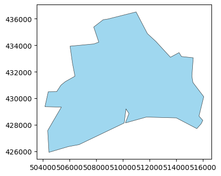
# The coordinate information in the geometry column of gdf_uk_la_2 has been changed from degree to meter.
# We can observe that the shape of the projected map (CRS is OSGB36 / British National Grid) is slightly different from the original map (CRS is WGS 84).
gdf_uk_la_2[gdf_uk_la_2["LAD24NM"] == "Kingston upon Hull, City of"].plot(color="skyblue", edgecolor="black", lw= 0.5, alpha=0.8, figsize=(6, 4))

<Axes: >

Q5 solution:

# Save the 'Kingston upon Hull, City of' boundary as 'Kingston_upon_Hull_boundary.geojson' in the data folder.
gdf_uk_la[gdf_uk_la["LAD24NM"] == "Kingston upon Hull, City of"].to_file("data/Kingston_upon_Hull_boundary.geojson", driver="GeoJSON")

Q6 solution:

# Save the 'Kingston upon Hull, City of' boundary as 'Kingston_upon_Hull_boundary.shp' in the data folder.
gdf_uk_la_2[gdf_uk_la_2["LAD24NM"] == "Kingston upon Hull, City of"].to_file("data/Kingston_upon_Hull_boundary.shp", driver="ESRI Shapefile")