Week4 Lab Tutorial Timeline

Time	Activity
16:00–16:05	Introduction — Overview of the main tasks for the lab tutorials
16:05–16:45	Tutorial: Spatial patterns 1 — Follow Section 4.1-4.2 of the Jupyter Notebook to practice the spatial weights and global spatial autocorrelation
16:45–17:30	Tutorial: Spatial patterns 2 — Follow Section 4.3-4.4 of the Jupyter Notebook to practice the local spatial autocorrelation and KDE
17:30–17:55	Quiz — Complete quiz tasks
17:55–18:00	Wrap-up — Recap key points and address final questions

For this module’s lab tutorials, you can download all the required data using the provided link (click).

Please make sure that both the Jupyter Notebook file and the data and img folder are placed in the same directory (specifically within the STBDA_lab folder) to ensure the code runs correctly.

Week 4 Key Takeaways:

• Understand the concept of spatial dependence and spatial autocorrelation.

• Compute spatial weights using different methods.

• Compute global spatial autocorrelation using Moran’s I.

• Compute local spatial autocorrelation using Local Moran’s I and Getis-Ord Gi*.

• Implement Kernel Density Estimation (KDE) to visualize spatial patterns.

4 Spatial patterns analysis

Spatial dependence is the phenomenon where the value of a variable at one location is influenced by the values of the same variable at nearby or neighboring locations (Near things are more related than distant things.— based on Tobler’s First Law of Geography).

If spatial data are sampled at nearby locations, they tend to be correlated with one another. In other words, Spatial dependence is a fundamental concept in spatial analysis and is often quantified using measures of spatial autocorrelation.

The phenomena of spatial dependence can be observed in the real world, for example, the population density of a city is likely to be similar in nearby neighborhoods, but different in neighborhoods that are far apart; or the rainfall in a region is likely to be similar in nearby areas, but different in areas that are far apart.

Autocorrelation is the correlation of a variable (or series) with itself.

Spatial autocorrelation is a statistical measure of the degree to which spatial dependence exists in the data. It’s a quantified outcome that shows how strongly (and in what way) spatial dependence appears. It can be positive (similar values are clustered together), negative (dissimilar values are clustered together), or zero (no spatial pattern).

4.1 Spatial Weights

A spatial weight matrix (spatial adjacency matrix) \(W\) is a square matrix that quantifies the spatial relationship between each pair of locations (\(i\) and \(j\) are the spatial unit index) across \(n\) spatial units:

\[\begin{split}W = \begin{bmatrix} w_{11} & w_{12} & \dots & w_{1n} \\ w_{21} & w_{22} & \dots & w_{2n} \\ \vdots & \vdots & \ddots & \vdots \\ w_{n1} & w_{n2} & \dots & w_{nn} \end{bmatrix}\end{split}\]

• \(w_{ij}\) is the spatial weight between location \(i\) and \(j\);

• Typically, \(w_{ii} = 0\) (no self-weight).

For example, if we have 4 areas/locations (A, B, C, D) with the index (1, 2, 3, 4) and the following spatial weight matrix can be \(W\): $$ W =

(1)\[\begin{bmatrix} w_{11} & w_{12} & w_{13} & w_{14} \\ w_{21} & w_{22} & w_{23} & w_{24} \\ w_{31} & w_{32} & w_{33} & w_{34} \\ w_{41} & w_{42} & w_{43} & w_{44} \end{bmatrix}\]

$$

How to compute the spatial weigt \(w_{i,j}\): we can list a tabel to show the different types of computing the spatial weight \(w_{i,j}\):

Type of spatial weight	Description	Formula	Value type
Contiguity (Queen)	Based on the adjacency of spatial units	\(w_{i,j} = 1\) if \(i\) and \(j\) are neighbors (for polygons, neighbors share an edge or corner), else \(0\)	Binary
Contiguity (Rook)	Based on the adjacency of spatial units	\(w_{i,j} = 1\) if \(i\) and \(j\) are neighbors (for polygons, neighbors share only an edge), else \(0\)	Binary
Distance	Based on the distance between spatial units	\(w_{i,j} = \frac{1}{d_{i,j}}\) if \(d_{i,j} < d_{threshold}\), else \(0\)	Binary
K-nearest neighbors	Based on the distance to the \(k\) nearest neighbors	\(w_{i,j} = 1\) if \(j\) is one of the \(k\) nearest neighbors of \(i\), else \(0\)	Binary
Inverse distance	Based on the inverse of the distance between spatial units	\(w_{i,j} = \frac{1}{d_{i,j}^k}\) if \(d_{i,j} < d_{threshold}\), else \(0\)	Continuous
Row-standardized	Based on the row-standardization of the spatial weight matrix	\(w_{i,j} = \frac{w_{i,j}}{\sum_j w_{i,j}}\)	Continuous
Column-standardized	Based on the column-standardization of the spatial weight matrix	\(w_{i,j} = \frac{w_{i,j}}{\sum_i w_{i,j}}\)	Continuous
Symmetric	Based on the symmetric standardization of the spatial weight matrix	\(w_{i,j} = \frac{w_{i,j}}{\sum_i w_{i,j} + \sum_j w_{i,j}}\)	Continuous

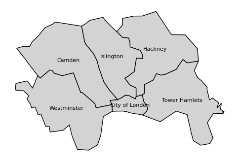
Now, we use the libpysal library to compute the spatial weights for selected central London boroughs/LAs (polygons).

# Import the required libraries
import geopandas as gpd
import libpysal.weights as weights
import matplotlib.pyplot as plt
import contextily as cx
import pandas as pd
import warnings

from spreg import white

warnings.filterwarnings("ignore")

# read the shapefile
gdf_uk_la = gpd.read_file('data/Local_Authority_Districts_December_2024_Boundaries_UK_BSC.geojson')
list_las_c_london = ['Camden', 'Hackney', 'Islington', 'Tower Hamlets', 'City of London', 'Westminster']
# Filter the GeoDataFrame to include only the inner London boroughs
gdf_c_london = gdf_uk_la[gdf_uk_la['LAD24NM'].isin(list_las_c_london)]
# transform the CRS to EPSG:27700 (British National Grid)
gdf_c_london = gdf_c_london.to_crs(epsg=27700)
gdf_c_london

	FID	LAD24CD	LAD24NM	LAD24NMW	BNG_E	BNG_N	LONG	LAT	GlobalID	geometry
263	264	E09000001	City of London		532382	181358	-0.09352	51.51564	741710fd-03e1-4b41-8645-7ebcfc5961ac	POLYGON ((533404.882 182037.774, 533534.125 18...
269	270	E09000007	Camden		527491	184283	-0.16291	51.54305	88f3f650-53ac-434d-883e-6235b48d14c4	POLYGON ((529150.075 185862.023, 529701.341 18...
274	275	E09000012	Hackney		534560	185787	-0.06046	51.55493	a41cf0fc-95ed-4823-a9db-7b8bc60f421b	POLYGON ((537570.535 185494.637, 537638.712 18...
281	282	E09000019	Islington		531160	184645	-0.10990	51.54547	43a872fc-e401-45af-a2e6-3b2befc98837	POLYGON ((533382.221 185149.793, 533460.932 18...
292	293	E09000030	Tower Hamlets		536340	181452	-0.03648	51.51555	54f82e61-dc15-42cb-b777-681b4326f855	POLYGON ((536480.759 184698.334, 536779.206 18...
295	296	E09000033	Westminster		528268	180871	-0.15295	51.51222	a52ff0f8-4ac0-4417-8338-01be3cbb516a	POLYGON ((526773.283 183663.262, 527373.359 18...

# plot the inner London boroughs
fig, ax = plt.subplots(figsize=(6, 6))
gdf_c_london.plot(ax=ax, color='lightgrey', edgecolor='black')
# set each name for the borough
for x, y, label in zip(gdf_c_london.geometry.centroid.x, gdf_c_london.geometry.centroid.y, gdf_c_london['LAD24NM']):
    ax.text(x, y, label, fontsize=8, ha='center', va='center')
ax.axis('off')
plt.show()

# set the index to the LAD24NM column
gdf_c_london.index = gdf_c_london['LAD24NM']
gdf_c_london.index

Index(['City of London', 'Camden', 'Hackney', 'Islington', 'Tower Hamlets',
       'Westminster'],
      dtype='object', name='LAD24NM')

Contiguity – Queen method

# Compute the spatial weights using the Queen contiguity method
w_q = weights.Queen.from_dataframe(gdf_c_london, use_index='True')
# the numbers of units
print('the numbers of units', w_q.n)

the numbers of units 6

# print the spatial weights df
df_wq = w_q.to_adjlist(drop_islands=True)
df_wq

	focal	neighbor	weight
0	City of London	Camden	1.0
1	City of London	Hackney	1.0
2	City of London	Islington	1.0
3	City of London	Tower Hamlets	1.0
4	City of London	Westminster	1.0
5	Camden	City of London	1.0
6	Camden	Islington	1.0
7	Camden	Westminster	1.0
8	Hackney	City of London	1.0
9	Hackney	Islington	1.0
10	Hackney	Tower Hamlets	1.0
11	Islington	City of London	1.0
12	Islington	Camden	1.0
13	Islington	Hackney	1.0
14	Tower Hamlets	City of London	1.0
15	Tower Hamlets	Hackney	1.0
16	Westminster	City of London	1.0
17	Westminster	Camden	1.0

# we can transfer the spatial weights list (df_wq) to spatial weight/adjacency matrix in pandas
df_wq_matrix = df_wq.pivot(index='focal', columns='neighbor', values='weight').fillna(0)
df_wq_matrix

neighbor	Camden	City of London	Hackney	Islington	Tower Hamlets	Westminster
focal
Camden	0.0	1.0	0.0	1.0	0.0	1.0
City of London	1.0	0.0	1.0	1.0	1.0	1.0
Hackney	0.0	1.0	0.0	1.0	1.0	0.0
Islington	1.0	1.0	1.0	0.0	0.0	0.0
Tower Hamlets	0.0	1.0	1.0	0.0	0.0	0.0
Westminster	1.0	1.0	0.0	0.0	0.0	0.0

# we can use .neighbors to get the neighbors of each unit
w_q.neighbors['Camden']

['Westminster', 'Islington', 'City of London']

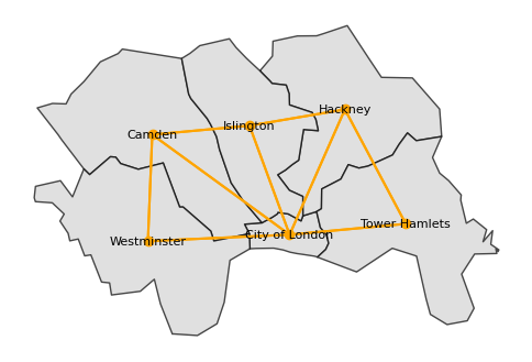
We can also plot the spatial weights using a network/graph representation, where the nodes represent the spatial units and the edges represent the spatial weights, here, if the two units are neighbors, the edge is drawn between them.

#plot the spatial weights using a network/graph representation
fig, ax = plt.subplots(figsize=(6, 6))
gdf_c_london.plot(ax=ax, color='lightgrey', edgecolor='black', alpha=0.7)
# set each name for the borough
for x, y, label in zip(gdf_c_london.geometry.centroid.x, gdf_c_london.geometry.centroid.y, gdf_c_london['LAD24NM']):
    ax.text(x, y, label, fontsize=8, ha='center', va='center')
ax.axis('off')
w_q.plot(gdf_c_london, ax=ax, color='orange')
plt.show()

Distance-based method

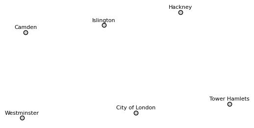
Distance-based spatial weights are based on the distance between spatial units, usually, the point locations. So, we transform the polygons to points (centroids) and then compute the distance-based spatial weights.

# transform the polygons to points (centroids)
gdf_c_london['geometry'] = gdf_c_london.geometry.centroid
# now six LAs are represented by their centroids/points
gdf_c_london

	FID	LAD24CD	LAD24NM	LAD24NMW	BNG_E	BNG_N	LONG	LAT	GlobalID	geometry
LAD24NM
City of London	264	E09000001	City of London		532382	181358	-0.09352	51.51564	741710fd-03e1-4b41-8645-7ebcfc5961ac	POINT (532493.308 181259.574)
Camden	270	E09000007	Camden		527491	184283	-0.16291	51.54305	88f3f650-53ac-434d-883e-6235b48d14c4	POINT (527843.276 184641.457)
Hackney	275	E09000012	Hackney		534560	185787	-0.06046	51.55493	a41cf0fc-95ed-4823-a9db-7b8bc60f421b	POINT (534363.476 185492.867)
Islington	282	E09000019	Islington		531160	184645	-0.10990	51.54547	43a872fc-e401-45af-a2e6-3b2befc98837	POINT (531135.378 184944.643)
Tower Hamlets	293	E09000030	Tower Hamlets		536340	181452	-0.03648	51.51555	54f82e61-dc15-42cb-b777-681b4326f855	POINT (536424.392 181625.502)
Westminster	296	E09000033	Westminster		528268	180871	-0.15295	51.51222	a52ff0f8-4ac0-4417-8338-01be3cbb516a	POINT (527697.219 181041.502)

# plot the centroids of the inner London boroughs
fig, ax = plt.subplots(figsize=(6, 6))
gdf_c_london.plot(ax=ax, color='lightgrey', edgecolor='black')
# set each name for the borough
for x, y, label in zip(gdf_c_london.geometry.x, gdf_c_london.geometry.y, gdf_c_london['LAD24NM']):
    ax.text(x, y+200, label, fontsize=8, ha='center', va='center')
ax.axis('off')
plt.show()

# Compute the spatial weights using the distance-based method, the threshold with 5000 means 5000 meters as the CRS is EPSG:27700
w_d = weights.DistanceBand.from_dataframe(gdf_c_london, threshold=5000, binary=True, use_index='True')

df_wd = w_d.to_adjlist(drop_islands=True)
df_wd

	focal	neighbor	weight
0	City of London	Hackney	1.0
1	City of London	Islington	1.0
2	City of London	Tower Hamlets	1.0
3	City of London	Westminster	1.0
4	Camden	Islington	1.0
5	Camden	Westminster	1.0
6	Hackney	City of London	1.0
7	Hackney	Islington	1.0
8	Hackney	Tower Hamlets	1.0
9	Islington	City of London	1.0
10	Islington	Camden	1.0
11	Islington	Hackney	1.0
12	Tower Hamlets	City of London	1.0
13	Tower Hamlets	Hackney	1.0
14	Westminster	City of London	1.0
15	Westminster	Camden	1.0

df_wd_matrix = df_wd.pivot(index='focal', columns='neighbor', values='weight').fillna(0)
df_wd_matrix

neighbor	Camden	City of London	Hackney	Islington	Tower Hamlets	Westminster
focal
Camden	0.0	0.0	0.0	1.0	0.0	1.0
City of London	0.0	0.0	1.0	1.0	1.0	1.0
Hackney	0.0	1.0	0.0	1.0	1.0	0.0
Islington	1.0	1.0	1.0	0.0	0.0	0.0
Tower Hamlets	0.0	1.0	1.0	0.0	0.0	0.0
Westminster	1.0	1.0	0.0	0.0	0.0	0.0

Inverse distance method

Compute the spatial weights using the inverse distance-based method, we need to set the binary parameter to False to get the continuous weights, then the weights are computed with a parameter alpha which is the power of the distance, if we set alpha = -1, then the weights are computed as \(w_{i,j} = \frac{1}{d_{i,j}}\).

alpha: distance decay parameter for weight (default -1.0) if alpha is positive the weights will not decline with distance.

# Compute the spatial weights using the inverse distance-based method, the threshold with 5000 means 5000 meters as the CRS is EPSG:27700
w_inverse_d = weights.DistanceBand.from_dataframe(gdf_c_london, threshold=5000, binary=False, alpha= -1, use_index='True')

df_w_in_d = w_inverse_d.to_adjlist(drop_islands=True)
df_w_in_d

	focal	neighbor	weight
0	City of London	Hackney	0.000216
1	City of London	Islington	0.000255
2	City of London	Tower Hamlets	0.000253
3	City of London	Westminster	0.000208
4	Camden	Islington	0.000302
5	Camden	Westminster	0.000278
6	Hackney	City of London	0.000216
7	Hackney	Islington	0.000305
8	Hackney	Tower Hamlets	0.000228
9	Islington	City of London	0.000255
10	Islington	Camden	0.000302
11	Islington	Hackney	0.000305
12	Tower Hamlets	City of London	0.000253
13	Tower Hamlets	Hackney	0.000228
14	Westminster	City of London	0.000208
15	Westminster	Camden	0.000278

df_w_in_d_matrix = df_w_in_d.pivot(index='focal', columns='neighbor', values='weight').fillna(0)
df_w_in_d_matrix

neighbor	Camden	City of London	Hackney	Islington	Tower Hamlets	Westminster
focal
Camden	0.000000	0.000000	0.000000	0.000302	0.000000	0.000278
City of London	0.000000	0.000000	0.000216	0.000255	0.000253	0.000208
Hackney	0.000000	0.000216	0.000000	0.000305	0.000228	0.000000
Islington	0.000302	0.000255	0.000305	0.000000	0.000000	0.000000
Tower Hamlets	0.000000	0.000253	0.000228	0.000000	0.000000	0.000000
Westminster	0.000278	0.000208	0.000000	0.000000	0.000000	0.000000

This distance-based with band/ thereshold of 5000 meters means that if the distance between two units is less than 5000 meters, then they are neighbors. This brings us a different spatial weight matrix compared to the contiguity queen method. When we check the neighbors of Camden in the distance-based method, only Islinton and Westminster points are its neighbors as they are within 5000 meters to the point of Camden.

w_d.neighbors['Camden']

['Islington', 'Westminster']

Note that there are lots of different ways to compute the spatial weights based on different data formats (not only the GeoDataframe). you can find some other functions in the libpysal library in this Page (click) and a general tutorial.

4.2 Global Spatial Autocorrelation

Global spatial autocorrelation answers the question: Is there overall clustering across the whole map?

Global Moran’s I :

Moran’s I (Moran, 1950) is a measure of global spatial autocorrelation. It is a single value that summarizes the degree of spatial autocorrelation in the entire dataset:

\[ I = \frac{n}{W} \cdot \frac{\sum_i \sum_j w_{ij} (x_i - \bar{x})(x_j - \bar{x})}{\sum_i (x_i - \bar{x})^2} \]

Where:

• \( n \): Number of spatial units

• \( x_i \): Value at location \( i \)

• \( \bar{x} \): Mean of the variable

• \( w_{ij} \): Spatial weight between location \( i \) and \( j \)

• \( W = \sum_i \sum_j w_{ij} \): Sum of all spatial weights

\(I > 0\): Positive spatial autocorrelation.

\(I < 0\): Negative spatial autocorrelation.

\(I = 0\): No spatial autocorrelation.

# Import the required libraries
import esda

Now, we will use the England LA with population data to compute the global Moran’s I for population density.

# the population data is in the `data` folder
df_pop = gpd.read_file('data/populaiton_2022_all_ages_uk.csv')

# merge the population data with the GeoDataFrame
gdf_uk_la_pop = pd.merge(gdf_uk_la, df_pop, left_on='LAD24CD', right_on='Code', how='left')

# select the england LAs
gdf_england_la_pop = gdf_uk_la_pop[gdf_uk_la_pop['LAD24CD'].str.startswith('E')]
# transform the CRS to EPSG:27700 (British National Grid)
gdf_england_la_pop = gdf_england_la_pop.to_crs(epsg=27700)
# rename the columns
gdf_england_la_pop = gdf_england_la_pop.rename(columns={'All ages': 'Population'})
gdf_england_la_pop['Population'] = gdf_england_la_pop['Population'].astype('int')
# calculate the population density: population per square kilometer
gdf_england_la_pop['Population_density'] = gdf_england_la_pop.apply(lambda x: x['Population']/ (x.geometry.area/1000000), axis=1)
gdf_england_la_pop

	FID	LAD24CD	LAD24NM	LAD24NMW	BNG_E	BNG_N	LONG	LAT	GlobalID	geometry	Code	Name	Geography	Population	Population_density
0	1	E06000001	Hartlepool		447161	531473	-1.27017	54.67613	fcc85d99-da7a-440c-aa80-b6e2a5353efe	POLYGON ((447851.213 537036.01, 448290.115 536...	E06000001	Hartlepool	Unitary Authority	93861	994.428583
1	2	E06000002	Middlesbrough		451141	516887	-1.21100	54.54468	0d2753c9-b44b-44e2-9b20-f70fd8a63e1a	POLYGON ((450791.114 520932.509, 450530.512 52...	E06000002	Middlesbrough	Unitary Authority	148285	2735.466726
2	3	E06000003	Redcar and Cleveland		464330	519596	-1.00657	54.56752	91793ade-9ca5-46dc-8591-7bd7fb61b233	POLYGON ((456987.212 526324.904, 459206.816 52...	E06000003	Redcar and Cleveland	Unitary Authority	137175	561.248283
3	4	E06000004	Stockton-on-Tees		444940	518179	-1.30665	54.55688	ae16dbb0-8ebe-49c6-bff9-f3479669fd4f	POLYGON ((445378.413 526449.708, 445536.511 52...	E06000004	Stockton-on-Tees	Unitary Authority	199966	976.155131
4	5	E06000005	Darlington		428029	515648	-1.56836	54.53534	f21d0ade-ae2f-4bff-9d85-1048cd649b5f	POLYGON ((423240.211 524970.902, 423783.816 52...	E06000005	Darlington	Unitary Authority	109469	553.554052
...	...	...	...	...	...	...	...	...	...	...	...	...	...	...	...
291	292	E09000029	Sutton		527357	163639	-0.17227	51.35755	1b5d57bc-1cb5-43e1-85ba-3bb45da0b7cc	POLYGON ((527423.64 167442.817, 527757.283 167...	E09000029	Sutton	London Borough	210053	4757.046484
292	293	E09000030	Tower Hamlets		536340	181452	-0.03648	51.51555	54f82e61-dc15-42cb-b777-681b4326f855	POLYGON ((536480.759 184698.334, 536779.206 18...	E09000030	Tower Hamlets	London Borough	325789	16494.761141
293	294	E09000031	Waltham Forest		537328	190278	-0.01880	51.59462	97cd624f-2c02-4f12-a78e-7aedc777673f	POLYGON ((539923.888 193889.058, 539562.889 19...	E09000031	Waltham Forest	London Borough	275887	7119.047670
294	295	E09000032	Wandsworth		525152	174138	-0.20022	51.45240	9c51587a-4315-449d-bcc7-e65625e402f7	POLYGON ((528637.184 175213.943, 528758.922 17...	E09000032	Wandsworth	London Borough	329035	9499.579457
295	296	E09000033	Westminster		528268	180871	-0.15295	51.51222	a52ff0f8-4ac0-4417-8338-01be3cbb516a	POLYGON ((526773.283 183663.262, 527373.359 18...	E09000033	Westminster	London Borough	211365	9843.368835

296 rows × 15 columns

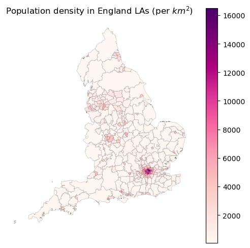
# plot the population data
fig, ax = plt.subplots(figsize=(6, 6))
gdf_england_la_pop.plot(column='Population_density', ax=ax, legend=True, cmap='RdPu', edgecolor='black', linewidth=0.1)
ax.axis('off')
plt.title('Population density in England LAs (per $km^2$)')
plt.show()

# compute the spatial weights using the Queen contiguity method
w_england_la_pop = weights.Queen.from_dataframe(gdf_england_la_pop, use_index='True')

# print the islands
for i in w_england_la_pop.islands:
    print(gdf_england_la_pop.loc[i, 'LAD24NM'])

Isle of Wight
Isles of Scilly

# compute the global Moran's I
mi = esda.Moran(gdf_england_la_pop['Population_density'], w_england_la_pop, two_tailed=True)

('WARNING: ', 43, ' is an island (no neighbors)')
('WARNING: ', 49, ' is an island (no neighbors)')

print('Moran\'s I:', mi.I)
print('p-value:', mi.p_sim)

Moran's I: 0.6242014303262433
p-value: 0.001

Interpretation of the Moran’s I: the result of the Moran’s I is 0.62, which indicates a positive spatial autocorrelation, meaning that the population density in England LAs is Strongly clustered together. The p-value is under 0.05, which indicates that the result is statistically significant at the 0.05 level. We can use the mi.sim to get the distribution of the Moran’s I under the null hypothesis of no spatial autocorrelation. You can find more details about the Moran’s I in the libpysal Moran documentation.

4.3 Local Spatial Autocorrelation / Association

Local spatial autocorrelation answers the questions: Is there clustering in a specific area? Which specific areas are clustered or are spatial outlier?

LISA (Local Indicators of Spatial Association) is a statistical technique that decomposes global spatial autocorrelation measures into location-specific contributions. It identifies significant spatial clusters or spatial outliers by measuring the correlation between a location and its neighbors.

Key aspects of LISA:

• Helps identify local patterns of spatial association (clusters and outliers)

• Indicates areas with significant high or low values

• Shows locations with similar or dissimilar values among neighbors

• Common LISA statistics include Local Moran’s I and Getis-Ord Gi*

• Useful for finding hot spots, cold spots, and spatial outliers

• Can be visualized through significance maps and cluster maps

4.3.1 Local Moran’s I

Local Moran’s I is a measure of local spatial autocorrelation. It is a value for each spatial unit that summarizes the degree of spatial autocorrelation in the local neighborhood of that unit:

\[ I_i = \frac{(x_i - \bar{x})}{S^2} \cdot \sum_j w_{ij} (x_j - \bar{x}) \]

Where:

• \( I_i \): Local Moran’s I for location \( i \) , (\( I_i \in (-\infty, +\infty) \))

• \( x_i \): Value at location \( i \)

• \( \bar{x} \): Mean of the variable

• \( S\): Standard deviation of the variable

• \( S^2 \): Variance of the variable

• \( w_{ij} \): Spatial weight between location \( i \) and \( j \)

• \( j \): Neighbors of location \( i \)

Interpretation:

\( I_i > 0 \): Positive spatial autocorrelation (high values surrounded by high values or low values surrounded by low values)

\(I_i < 0 \): Negative spatial autocorrelation (high values surrounded by low values or low values surrounded by high values)

\(I_i = 0 \): No spatial autocorrelation

We continue to use the England LA with population data to compute the local Moran’s I.

# compute the local Moran's I
lm = esda.Moran_Local(gdf_england_la_pop['Population_density'], w_england_la_pop)

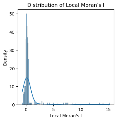
Note that the local Moran’s I is a distribution of values, not a single value like the global Moran’s I. The local Moran’s I can be used to identify the spatial clusters and outliers in the data.

# plot the distribution of local Moran's I using histogram and kde by seaborn
import seaborn as sns
fig, ax = plt.subplots(figsize=(4, 4))
sns.histplot(lm.Is, kde=True, ax=ax)
ax.set_xlabel('Local Moran\'s I')
ax.set_ylabel('Density')
ax.set_title('Distribution of Local Moran\'s I')
plt.show()

For a better visualization, we should set the vmin and vmax in gdf.plot() to the min and max of the local Moran’s I value for building the colormap. This can make sure that the 0 is at the middle of the diverging colormap showing while color, and the color is symmetric to show the positive and negative values.

# mapping the local Moran's I
gdf_england_la_pop['local_moran'] = lm.Is
gdf_england_la_pop['p_value'] = lm.p_sim
gdf_england_la_pop['local_moran'] = gdf_england_la_pop['local_moran'].astype('float')
gdf_england_la_pop['local_moran'] = gdf_england_la_pop['local_moran'].fillna(0)
# plot the local Moran's I
fig, ax = plt.subplots(figsize=(8, 8))
# set the area with p values >=0.05 as the white
gdf_england_la_pop[~(gdf_england_la_pop['p_value'] < 0.05)].plot(ax=ax,color='white',edgecolor='black',linewidth=0.05)
# set the area with p values <0.05 with cmap
gdf_england_la_pop[gdf_england_la_pop['p_value'] < 0.05].plot(column='local_moran', ax=ax, legend=True,
                        cmap='seismic',
                        vmin=-15, vmax=15, # set the vmin and vmax to the min and max of the local Moran's I for cmap
                        edgecolor='black',
                        linewidth=0.05)
ax.axis('off')
# set the title
plt.title('Local Moran\'s I for Population Density in England LAs')
plt.show()

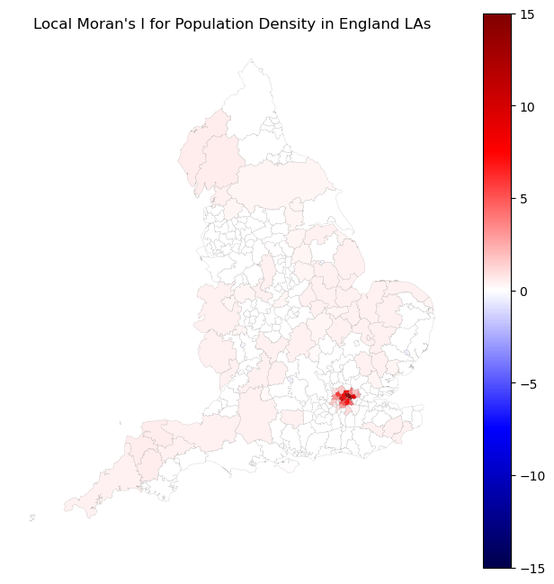
rendering: In the map, the red areas indicate high-high clusters (high population surrounded by high population), and the blue areas indicate low-low clusters (low population surrounded by low population). The white areas indicate outliers (high population surrounded by low population or low population surrounded by high population). We can found that the London boroughs are high-high clusters, and the areas in the north of England are low-low clusters.

You can find more details about the Local Moran’s I in the libpysal Local Moran I documentation.

4.3.2 Getis-Ord Gi*

Getis-Ord Gi* is a measure of local spatial autocorrelation that identifies clusters of high or low values. It is similar to Local Moran’s I, but it is more sensitive to the presence of outliers. It is used to identify hot spots (high values) and cold spots (low values) in the data:

\[ G_i^* = \frac{\sum_{j=1}^{n} w_{ij} x_j - \bar{x} \sum_{j=1}^{n} w_{ij}} {S \sqrt{\frac{n \sum_{j=1}^{n} w_{ij}^2 - \left( \sum_{j=1}^{n} w_{ij} \right) ^2 } {n - 1}}} \]

Where:

• \(G_i^*\): Getis-Ord Gi* index/value

• \( x_j \): Value at location \( j \)

• \( n \): the numbers of spatial units

• \( \bar{x} \): Mean of the variable

• \( S\): Standard deviation of the variable

• \( w_{ij} \): Spatial weight between location \( i \) and \( j \)

• \( j \): Neighbors of location \( i \)

Interpretation:

The \( G_i^* \) statistic is a z-score that indicates the presence of spatial clusters (hot or cold spots) around a location \( i \).

• \( G_i^* > 0 \): Indicates clustering of high values near location –> Hot spot if p <0.05.

• \( G_i^* < 0 \): Indicates clustering of low values near location \( i \) –> Cold spot if p <0.05.

• \( G_i^* \approx 0 \): No significant clustering around location \( i \) –> Spatial randomness.

Note: The raw G statistic measures the spatial association of neighboring values excluding the value at the location itself.

\[ G_i = \frac{ \sum_{j \ne i} w_{ij} x_j }{ \sum_{j} x_j } \]

We can use the esda library as a part of pysal to compute the Getis-Ord Gi* for detecting crime hotspots in London. Here we use the new spatial unit of analysis from UK census, which called LSOA (Lower Layer Super Output Area) which is a small area of about 1500 people on average in the UK. Crime data is from UK police open data, and LSOA boundary data is from ONS.

# read the lsoa boundary data of England and Wales
gdf_lsoa_uk = gpd.read_file('data/Lower_layer_Super_Output_Areas_(December_2021)_Boundaries_EW_BFC_(V10).geojson')
gdf_lsoa_uk

	FID	LSOA21CD	LSOA21NM	LSOA21NMW	BNG_E	BNG_N	LAT	LONG	Shape__Area	Shape__Length	GlobalID	geometry
0	1	E01000001	City of London 001A		532123	181632	51.51817	-0.097150	1.298653e+05	2635.767993	c625aea8-6d73-4b2a-be76-4d5c44cad9f8	POLYGON ((-0.09665 51.52028, -0.09663 51.52025...
1	2	E01000002	City of London 001B		532480	181715	51.51883	-0.091970	2.284198e+05	2707.816821	52c878e9-ac68-4886-b4a8-fea9cd241a70	POLYGON ((-0.08967 51.52069, -0.08971 51.52058...
2	3	E01000003	City of London 001C		532239	182033	51.52174	-0.095330	5.905420e+04	1224.573160	b9d8faca-d489-478d-8ce6-acaf76186d7d	POLYGON ((-0.0965 51.52295, -0.09644 51.52282,...
3	4	E01000005	City of London 001E		533581	181283	51.51469	-0.076280	1.895777e+05	2275.805344	15e1417d-537c-4845-9820-fc7596bd59b0	POLYGON ((-0.07568 51.51575, -0.07539 51.51555...
4	5	E01000006	Barking and Dagenham 016A		544994	184274	51.53875	0.089317	1.465370e+05	1966.092607	8a6c4ee0-c0ff-4736-9cfa-fb12a6d50da0	POLYGON ((0.09125 51.53905, 0.0915 51.5389, 0....
...	...	...	...	...	...	...	...	...	...	...	...	...
35667	35668	W01002036	Vale of Glamorgan 005G	Bro Morgannwg 005G	317939	172435	51.44494	-3.182180	3.886975e+05	3584.168435	5e3f978b-66c7-4828-a107-321cb22354e0	POLYGON ((-3.18412 51.44728, -3.18383 51.44727...
35668	35669	W01002037	Vale of Glamorgan 005H	Bro Morgannwg 005H	318527	172406	51.44476	-3.173710	2.843506e+05	3225.349982	b7aae689-c82d-4ddb-b899-4ba7918dac32	POLYGON ((-3.16647 51.44662, -3.16682 51.44628...
35669	35670	W01002038	Vale of Glamorgan 014G	Bro Morgannwg 014G	306491	167360	51.39754	-3.345520	3.495213e+06	12630.457940	144e5aed-4099-4dff-a48e-9f8c270d916b	POLYGON ((-3.34759 51.4098, -3.34771 51.40942,...
35670	35671	W01002039	Vale of Glamorgan 014H	Bro Morgannwg 014H	306564	166023	51.38553	-3.344120	6.505253e+05	3712.034400	bcf06740-abe0-4052-9ec2-7cad09d42195	POLYGON ((-3.34039 51.38935, -3.34035 51.38921...
35671	35672	W01002040	Vale of Glamorgan 015F	Bro Morgannwg 015F	311423	167179	51.39670	-3.274600	6.811834e+05	4888.403666	672a2fee-23b5-4a26-9a9d-901fc12f649e	POLYGON ((-3.26521 51.40005, -3.2652 51.40005,...

35672 rows × 12 columns

There are lots of methods to select the LSAOs for LAs.

• We can use the LA names to select the LSOAs ([‘LSOA21NM’]) from gdf_lsoa_uk;

• We can use the LSOA codes to select the LSOAs ([‘LSOA21CD’]) from gdf_lsoa_uk, but you need to check the LSOA codes in the LAs through the look_up file.

• We can use implement the sjoin between the LA geo boundary and LSOA boundary to select the LSOAs for LAs.

Here, We use the London LA names to select the LSOAs from gdf_lsoa_uk.

gdf_uk_london = gdf_uk_la[gdf_uk_la['LAD24CD'].str.startswith('E09')]
London_LA_names = gdf_uk_london.LAD24NM.unique()
print(London_LA_names)

['City of London' 'Barking and Dagenham' 'Barnet' 'Bexley' 'Brent'
 'Bromley' 'Camden' 'Croydon' 'Ealing' 'Enfield' 'Greenwich' 'Hackney'
 'Hammersmith and Fulham' 'Haringey' 'Harrow' 'Havering' 'Hillingdon'
 'Hounslow' 'Islington' 'Kensington and Chelsea' 'Kingston upon Thames'
 'Lambeth' 'Lewisham' 'Merton' 'Newham' 'Redbridge' 'Richmond upon Thames'
 'Southwark' 'Sutton' 'Tower Hamlets' 'Waltham Forest' 'Wandsworth'
 'Westminster']

'City of London 001E'

'City of London 001E'

# Extract the LA name from LSOA name (' '.join(x.split(' ')[:-1] as LSOA named as 'LA NAME 001A' ) and check if it's in London_LA_names
gdf_lsoa_uk['LA'] = gdf_lsoa_uk['LSOA21NM'].apply(lambda x: 'GL' if ' '.join(x.split(' ')[:-1]) in London_LA_names else 'NO')
# select the LSOAs in London
gdf_lsoa_london = gdf_lsoa_uk[gdf_lsoa_uk['LA'] == 'GL']
# transform the CRS to EPSG:27700 (British National Grid)
gdf_lsoa_london = gdf_lsoa_london.to_crs(epsg=27700)
# 4994 LSOAs in London
gdf_lsoa_london

	FID	LSOA21CD	LSOA21NM	LSOA21NMW	BNG_E	BNG_N	LAT	LONG	Shape__Area	Shape__Length	GlobalID	geometry	LA
0	1	E01000001	City of London 001A		532123	181632	51.51817	-0.097150	1.298653e+05	2635.767993	c625aea8-6d73-4b2a-be76-4d5c44cad9f8	POLYGON ((532151.55 181867.437, 532152.512 181...	GL
1	2	E01000002	City of London 001B		532480	181715	51.51883	-0.091970	2.284198e+05	2707.816821	52c878e9-ac68-4886-b4a8-fea9cd241a70	POLYGON ((532634.509 181926.019, 532632.06 181...	GL
2	3	E01000003	City of London 001C		532239	182033	51.52174	-0.095330	5.905420e+04	1224.573160	b9d8faca-d489-478d-8ce6-acaf76186d7d	POLYGON ((532153.715 182165.158, 532158.262 18...	GL
3	4	E01000005	City of London 001E		533581	181283	51.51469	-0.076280	1.895777e+05	2275.805344	15e1417d-537c-4845-9820-fc7596bd59b0	POLYGON ((533619.075 181402.367, 533639.881 18...	GL
4	5	E01000006	Barking and Dagenham 016A		544994	184274	51.53875	0.089317	1.465370e+05	1966.092607	8a6c4ee0-c0ff-4736-9cfa-fb12a6d50da0	POLYGON ((545126.865 184310.841, 545145.226 18...	GL
...	...	...	...	...	...	...	...	...	...	...	...	...	...
33711	33712	E01035718	Westminster 019G		527211	180107	51.50559	-0.168450	2.671900e+06	10740.132994	738fac0f-b4ee-47dc-a87c-2c0f8f147977	POLYGON ((528044.961 180617.988, 528046.356 18...	GL
33712	33713	E01035719	Westminster 021F		530127	178755	51.49277	-0.126960	9.294961e+04	2013.141792	7abdbf89-97f8-43f3-96b1-d162e667bed2	POLYGON ((530267.012 178811.303, 530265.762 17...	GL
33713	33714	E01035720	Westminster 021G		530009	178440	51.48997	-0.128770	1.061637e+05	2229.186337	653fb71a-b240-4e54-875d-0ec1f2f9cc2a	POLYGON ((529856.163 178761.75, 529856.871 178...	GL
33714	33715	E01035721	Westminster 023H		528403	178364	51.48965	-0.151920	2.168432e+05	2738.810595	ed04243a-989b-4bde-aeae-82d40ddffd10	POLYGON ((528641.829 178630.889, 528635.702 17...	GL
33715	33716	E01035722	Westminster 024G		529546	178076	51.48681	-0.135570	1.222497e+05	2211.190430	fd9bcb9b-a2e1-4381-a473-72bc1b5cf0c9	POLYGON ((529606.375 178302.448, 529606.654 17...	GL

4994 rows × 13 columns

# read the csvs in the data/police_met_city_2024 folder
import os
import glob
import pandas as pd

# get the csv files in the 2024-01 to 2014-12 folders in the data/police_met_city_2024 folder
path = 'data/police_met_city_2024'
# to get all the csv files in the path, "**/*.csv" means all the csv files in the subfolders; glob means to get the files in the path
all_files = glob.glob(os.path.join(path, "**/*.csv"), recursive=True)
# read the csv files and concatenate them into a single dataframe
df_crime = pd.concat((pd.read_csv(f) for f in all_files), ignore_index=True)
# we can save it to one csv file
# df_crime.to_csv('data/crime_2024_call_police_met_city.csv', index=False)

# check the columns
df_crime.head()
print(len(df_crime))

1149321

Now, we need conbime to df_crime (points) to gdf_lsoa_london (polygons), we can use sjoin to do this (or use the LSOA codes to do this).

# get gdf from the df_crime with x and y coordinates
gdf_crime = gpd.GeoDataFrame(df_crime, geometry=gpd.points_from_xy(df_crime['Longitude'], df_crime['Latitude']), crs='EPSG:4326')
# transform the CRS to EPSG:27700 (British National Grid)
gdf_crime = gdf_crime.to_crs(epsg=27700)
# spatial join the gdf_crime and gdf_lsoa_london
gdf_crime = gpd.sjoin(gdf_crime, gdf_lsoa_london, how='inner', predicate='intersects')

We can find there are 1,149,321 - 1,144,178 = 4,143 dropped as the pts are not intersected with the polygons.

# check the number of rows
len(gdf_crime)
# check the columns
gdf_crime.head()

	Crime ID	Month	Reported by	Falls within	Longitude	Latitude	Location	LSOA code	LSOA name	Crime type	...	LSOA21NM	LSOA21NMW	BNG_E	BNG_N	LAT	LONG	Shape__Area	Shape__Length	GlobalID	LA
0	b74d06161e2425ef2abf28345aa962fa862753669659d3...	2024-09	City of London Police	City of London Police	-0.107682	51.517786	On or near B521	E01000917	Camden 027C	Robbery	...	Camden 027C		531169	181859	51.52043	-0.11080	75063.537949	2405.390222	7205eeed-3cf1-4502-9073-4e8afb75ea58	GL
1	ab9f963604d03486ffbefec80f9f9296c7f65ecd4cd047...	2024-09	City of London Police	City of London Police	-0.107682	51.517786	On or near B521	E01000917	Camden 027C	Violence and sexual offences	...	Camden 027C		531169	181859	51.52043	-0.11080	75063.537949	2405.390222	7205eeed-3cf1-4502-9073-4e8afb75ea58	GL
2	7eaad3255f757cf5073dfd3712193f4497e788b3f6519f...	2024-09	City of London Police	City of London Police	-0.112096	51.515942	On or near Nightclub	E01000914	Camden 028B	Violence and sexual offences	...	Camden 028B		530733	181688	51.51899	-0.11715	448043.096497	4946.142062	9e7739b0-5ee1-4923-ad52-648147b8c13c	GL
3	71c1e6edfb73383e82ca6acdc1c9c0ef015334b529f298...	2024-09	City of London Police	City of London Police	-0.111596	51.518281	On or near Chancery Lane	E01000914	Camden 028B	Violence and sexual offences	...	Camden 028B		530733	181688	51.51899	-0.11715	448043.096497	4946.142062	9e7739b0-5ee1-4923-ad52-648147b8c13c	GL
4	06e7c6b6541166a8abe71de2593b9576c5e26215e349e4...	2024-09	City of London Police	City of London Police	-0.098519	51.517332	On or near Little Britain	E01000001	City of London 001A	Other theft	...	City of London 001A		532123	181632	51.51817	-0.09715	129865.314476	2635.767993	c625aea8-6d73-4b2a-be76-4d5c44cad9f8	GL

5 rows × 26 columns

Spatial and temporal aggregation of the data refers to the process of combining and summarizing data across different geographic areas (spatial) and time periods (temporal):

Spatial Aggregation:

• Combining data from smaller geographic units into larger areas

• Example: Aggregating crime incidents from LSOA level to London borough level

Temporal Aggregation:

• Combining data across different time periods

• Example: Converting daily crime data into monthly or yearly totals

# here we aggregate the all crime data to LSOA and month level using groupby
df_crime_agg = gdf_crime.groupby(['LSOA21CD', 'Month']).agg({'Crime ID': 'count'}).reset_index().rename(columns={'Crime ID': 'Count'})

# select May 2024 of all crimes for analysis
df_crime_agg_may = df_crime_agg[df_crime_agg['Month'] == '2024-05']

# check the columns
df_crime_agg_may

	LSOA21CD	Month	Count
4	E01000001	2024-05	11
16	E01000002	2024-05	38
28	E01000003	2024-05	13
40	E01000005	2024-05	72
52	E01000006	2024-05	10
...	...	...	...
59503	E01035718	2024-05	156
59515	E01035719	2024-05	9
59527	E01035720	2024-05	3
59539	E01035721	2024-05	61
59551	E01035722	2024-05	7

4965 rows × 3 columns

print('The numbers of LSOAs without crime in May 2024:', len(gdf_lsoa_london) - len(df_crime_agg_may))

The numbers of LSOAs without crime in May 2024: 29

# We use esda to compute the Getis-Ord Gi* for detecting crime hotspots in London.
# first, we need to merge the gdf_crime_agg_may with gdf_lsoa_london to get the geometry
gdf_crime_agg_may = pd.merge(gdf_lsoa_london[['LSOA21CD', 'geometry']], df_crime_agg_may, on='LSOA21CD', how='left')
# fill na
gdf_crime_agg_may = gdf_crime_agg_may.fillna(0)
gdf_crime_agg_may

	LSOA21CD	geometry	Month	Count
0	E01000001	POLYGON ((532151.55 181867.437, 532152.512 181...	2024-05	11.0
1	E01000002	POLYGON ((532634.509 181926.019, 532632.06 181...	2024-05	38.0
2	E01000003	POLYGON ((532153.715 182165.158, 532158.262 18...	2024-05	13.0
3	E01000005	POLYGON ((533619.075 181402.367, 533639.881 18...	2024-05	72.0
4	E01000006	POLYGON ((545126.865 184310.841, 545145.226 18...	2024-05	10.0
...	...	...	...	...
4989	E01035718	POLYGON ((528044.961 180617.988, 528046.356 18...	2024-05	156.0
4990	E01035719	POLYGON ((530267.012 178811.303, 530265.762 17...	2024-05	9.0
4991	E01035720	POLYGON ((529856.163 178761.75, 529856.871 178...	2024-05	3.0
4992	E01035721	POLYGON ((528641.829 178630.889, 528635.702 17...	2024-05	61.0
4993	E01035722	POLYGON ((529606.375 178302.448, 529606.654 17...	2024-05	7.0

4994 rows × 4 columns

# compute the spatial weights using the Queen contiguity method
w_lsoa_london = weights.Queen.from_dataframe(gdf_crime_agg_may, use_index='True')
# compute the Getis-Ord Gi* for the crime data
gi = esda.G_Local(gdf_crime_agg_may['Count'].values, w_lsoa_london)

# print the Getis-Ord Gi* values
gi.Zs

array([ 4.8966406 ,  6.05568957,  1.26792881, ..., -0.20360301,
        0.42941597, -0.17028329])

len(gi.Zs)

4994

# plot the distribution of Getis-Ord Gi* using histogram and kde by seaborn
fig, ax = plt.subplots(figsize=(4, 4))
sns.histplot(gi.Zs, kde=True, ax=ax)
ax.set_xlabel('Getis-Ord Gi*')
ax.set_ylabel('Density')

Text(0, 0.5, 'Density')

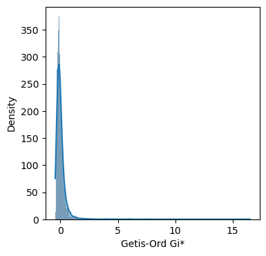
Z-scores: standardized G statistics that follow a normal distribution under spatial randomness.

P values: P-values from randomization/permutation.

# we can generate a df to show all the atrributes of the Getis-Ord Gi*
df_gi = pd.DataFrame({
    'Zs': gi.Zs,  # Z-scores: standardized G statistics that follow a normal distribution under spatial randomness
    'Gs': gi.Gs,  # Raw G statistics: measure of spatial concentration of attribute values (crime counts)
    'p_sim': gi.p_sim  # P-values from randomization
})
df_gi

	Zs	Gs	p_sim
0	4.896641	0.002149	0.001
1	6.055690	0.002611	0.001
2	1.267929	0.000705	0.012
3	3.965206	0.001779	0.001
4	-0.012130	0.000195	0.355
...	...	...	...
4989	1.016448	0.000605	0.006
4990	0.637040	0.000454	0.030
4991	-0.203603	0.000119	0.232
4992	0.429416	0.000371	0.050
4993	-0.170283	0.000133	0.308

4994 rows × 3 columns

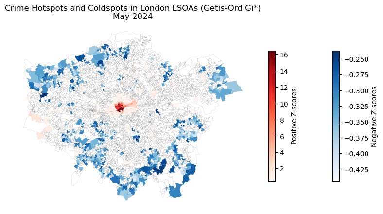
You can use any strategies to plot the gi resluts, here we can plot the results to the map with three parts:

• Hotspots: High positive Z-score (>0) with p-value < 0.05.

• Coldspots: High negative Z-score (<0) with p-value < 0.05.

• We usually use blank color to draw the ‘Not Significant cluster’ (p_value \(\geq\) 0.05).

# Add the Z-scores to the GeoDataFrame  
gdf_crime_agg_may['Z_score'] = gi.Zs
gdf_crime_agg_may['p_sim'] = gi.p_sim
# Create a figure and axis
fig, ax = plt.subplots(figsize=(10, 10))
# Plot not significant areas (p_sim >= 0.05)
gdf_crime_agg_may[gdf_crime_agg_may['p_sim'] >= 0.05].plot(
    ax=ax, color='white', edgecolor='black', linewidth=0.05)
# Plot cold spots (negative Z-scores and p_sim < 0.05)
gdf_crime_agg_may[(gdf_crime_agg_may['Z_score'] < 0) & (gdf_crime_agg_may['p_sim'] < 0.05)].plot(
    column='Z_score',
    ax=ax,
    cmap='Blues',
    legend=True,
    legend_kwds={'shrink': 0.35, 'orientation': 'vertical', 'label': 'Negative Z-scores',},
    linewidth=0.05)
# Plot hot spots (positive Z-scores and p_sim < 0.05)
gdf_crime_agg_may[(gdf_crime_agg_may['Z_score'] > 0) & (gdf_crime_agg_may['p_sim'] < 0.05)].plot(
    column='Z_score',
    ax=ax,
    cmap='Reds',
    legend=True,
    legend_kwds={'shrink': 0.35, 'orientation': 'vertical', 'label': 'Positive Z-scores'},
    linewidth=0.05)
ax.axis('off')
plt.title('Crime Hotspots and Coldspots in London LSOAs (Getis-Ord Gi*)\nMay 2024')
plt.show()

4.4 Kernel density estimation (KDE) analysis

Kernel Density Analysis (KDE) is a spatial analysis technique used to estimate the density of features (usually points or lines) across a surface. It creates a smooth, continuous surface that highlights areas of high and low concentration, often referred to as hotspots.

KDE function:

\[ \hat{f}(x) = \frac{1}{n h^2} \sum_{i=1}^{n} K\left(\frac{\|x - x_i\|}{h}\right) \]

• \( \hat{f}(x) \) is the estimated density at location \( x \), how “intense” the points are around location \(x\) (i.e., the ‘grid cell’ center or pixel).

• \( n \) is the total number of observations.

• \( h \) is the bandwidth (smoothing parameter). It controls the “spread” of the kernel. Larger \(h\) = smoother surface; smaller \(h\) = more detailed, but possibly noisy.

• \( h^2\): Since we are in 2D space, the area scaling is by \( h^2 \). In 1D, it’s just \(h\).

• \( x \): Target location where we estimate the density (i.e., the ‘grid cell’ center or pixel).

• \( x_i \): observed data point location.

• \( \|x - x_i\| \): Euclidean distance between location \(x\) and \(x_i\).

• \( K \) is the kernel function (e.g., Gaussian), which defines the shape of the influence of each point.

Gaussian KDE:

\[ K(u) = \frac{1}{2\pi} e^{-\frac{1}{2} u^2} \]

• \(u\): \(u = \|x - x_i\|\);

• \(e\): Euler’s number (~2.718), base of the natural exponential;

• \(e^{-\frac{1}{2} u^2}\): Gives the Gaussian bell curve shape;

• \(\frac{1}{2\pi}\): Normalization constant for 2D Gaussian;

gdf_crime.Month.unique()

array(['2024-09', '2024-07', '2024-06', '2024-01', '2024-08', '2024-12',
       '2024-04', '2024-03', '2024-02', '2024-05', '2024-11', '2024-10'],
      dtype=object)

gdf_crime_london_may = gdf_crime[gdf_crime['Month'] == '2024-05']
# transfer to web mercator
gdf_crime_london_may = gdf_crime_london_may.to_crs(epsg=3857)

gdf_crime_london_may

	Crime ID	Month	Reported by	Falls within	Longitude	Latitude	Location	LSOA code	LSOA name	Crime type	...	LSOA21NM	LSOA21NMW	BNG_E	BNG_N	LAT	LONG	Shape__Area	Shape__Length	GlobalID	LA
850782	eebfcc999f8ab6654adc6bc681e9ea2cd91c5026f895eb...	2024-05	City of London Police	City of London Police	-0.106345	51.520463	On or near Further/Higher Educational Building	E01000916	Camden 027B	Theft from the person	...	Camden 027B		531300	181907	51.52083	-0.10890	147250.335907	2272.325316	63388f71-c821-452f-bb92-dc8f74f031f3	GL
850783	67cbe410e90ad30207c925457c4d223e890f49dc7b394e...	2024-05	City of London Police	City of London Police	-0.106220	51.518275	On or near B500	E01000916	Camden 027B	Theft from the person	...	Camden 027B		531300	181907	51.52083	-0.10890	147250.335907	2272.325316	63388f71-c821-452f-bb92-dc8f74f031f3	GL
850784	a86f33f326d3d9a1f8c3972520e11717766029031efb90...	2024-05	City of London Police	City of London Police	-0.107682	51.517786	On or near B521	E01000917	Camden 027C	Drugs	...	Camden 027C		531169	181859	51.52043	-0.11080	75063.537949	2405.390222	7205eeed-3cf1-4502-9073-4e8afb75ea58	GL
850785	7a0554ddf2546c70556b59f8f7ca33099c3bd88fea79c7...	2024-05	City of London Police	City of London Police	-0.107682	51.517786	On or near B521	E01000917	Camden 027C	Other theft	...	Camden 027C		531169	181859	51.52043	-0.11080	75063.537949	2405.390222	7205eeed-3cf1-4502-9073-4e8afb75ea58	GL
850786	NaN	2024-05	City of London Police	City of London Police	-0.111596	51.518281	On or near Chancery Lane	E01000914	Camden 028B	Anti-social behaviour	...	Camden 028B		530733	181688	51.51899	-0.11715	448043.096497	4946.142062	9e7739b0-5ee1-4923-ad52-648147b8c13c	GL
...	...	...	...	...	...	...	...	...	...	...	...	...	...	...	...	...	...	...	...	...	...
948781	26f6034c0c51ca869a66a660a4cd3d9c548c6a48f5f7c6...	2024-05	Metropolitan Police Service	Metropolitan Police Service	-0.135320	51.487600	On or near St George'S Square	E01035722	Westminster 024G	Other theft	...	Westminster 024G		529546	178076	51.48681	-0.13557	122249.696388	2211.190430	fd9bcb9b-a2e1-4381-a473-72bc1b5cf0c9	GL
948782	ac16503056d8b26a3c0b4f407b7a632d8a4a2bee435838...	2024-05	Metropolitan Police Service	Metropolitan Police Service	-0.136284	51.485152	On or near Petrol Station	E01035722	Westminster 024G	Other theft	...	Westminster 024G		529546	178076	51.48681	-0.13557	122249.696388	2211.190430	fd9bcb9b-a2e1-4381-a473-72bc1b5cf0c9	GL
948783	88bf1a5d62b5201749e67773eb1108c13971d6f8067b86...	2024-05	Metropolitan Police Service	Metropolitan Police Service	-0.135320	51.487600	On or near St George'S Square	E01035722	Westminster 024G	Robbery	...	Westminster 024G		529546	178076	51.48681	-0.13557	122249.696388	2211.190430	fd9bcb9b-a2e1-4381-a473-72bc1b5cf0c9	GL
948784	3598323197468c36768d7a72a8015c721ec1a65fbd1bdf...	2024-05	Metropolitan Police Service	Metropolitan Police Service	-0.136284	51.485152	On or near Petrol Station	E01035722	Westminster 024G	Theft from the person	...	Westminster 024G		529546	178076	51.48681	-0.13557	122249.696388	2211.190430	fd9bcb9b-a2e1-4381-a473-72bc1b5cf0c9	GL
948785	19f7be6ed6c32479c4d138650ba5d19ee5c76144a390f1...	2024-05	Metropolitan Police Service	Metropolitan Police Service	-0.137230	51.486309	On or near Parking Area	E01035722	Westminster 024G	Violence and sexual offences	...	Westminster 024G		529546	178076	51.48681	-0.13557	122249.696388	2211.190430	fd9bcb9b-a2e1-4381-a473-72bc1b5cf0c9	GL

97636 rows × 26 columns

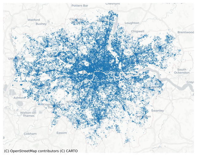
fig, ax = plt.subplots(figsize=(8, 8))
gdf_crime_london_may.plot(ax=ax, markersize=0.03)
cx.add_basemap(ax, crs="EPSG:3857", source=cx.providers.CartoDB.Positron, zoom=10)
ax.axis('off')
plt.show()

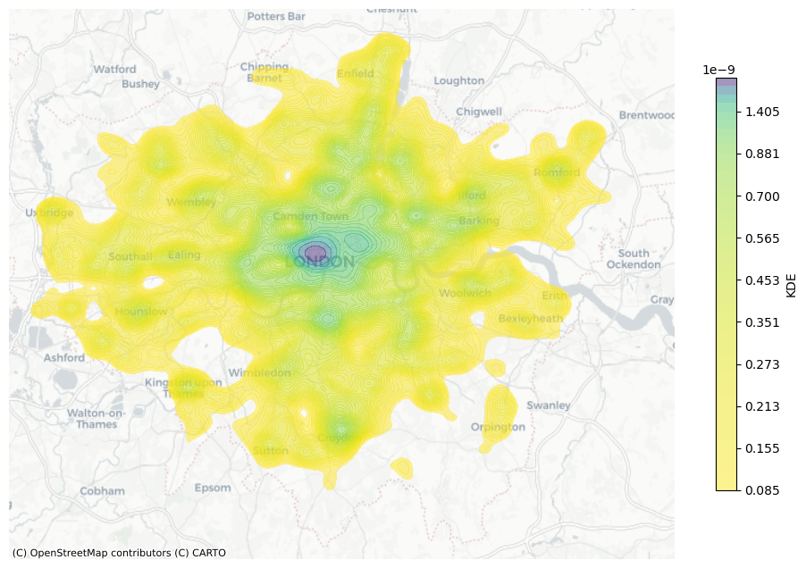
We use seaborn.kdeplot to plot the KDE analysis. in kedplot, it inherently use the gaussian_kde() in SciPy to caculate KDE, then it evaluates the KDE on the grid created.

fig, ax = plt.subplots(figsize=(12, 8))
kde = sns.kdeplot(ax=ax, x=gdf_crime_london_may.geometry.x,
            y=gdf_crime_london_may.geometry.y,
            n_levels=50, # how many contour lines or shaded bands are drawn in a 2D KDE plot
            shade=True,
            alpha=0.5,
            cmap="viridis_r",
            bw_adjust=0.6, # Adjust the bandwidth (lower values = narrower kernel)
            gridsize=300, # Number of points on each dimension of the evaluation grid.
             )
# Add colorbar manually
cbar = plt.colorbar(kde.collections[0], ax=ax, shrink=0.75)
cbar.set_label("KDE")
cx.add_basemap(ax, crs="EPSG:3857", source=cx.providers.CartoDB.Positron, zoom=10)
ax.axis('off')
plt.show()

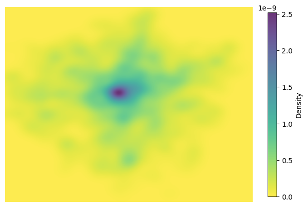
np.mgrid is a mesh-grid generator in NumPy. It creates coordinate matrices (grids) from coordinate vectors, typically used for evaluating functions over a 2D area.

from scipy.stats import gaussian_kde
import numpy as np
# Extract coordinates
x = gdf_crime_london_may.geometry.x
y = gdf_crime_london_may.geometry.y
point_xy = np.vstack([x, y]) # vertical stack in NumPy, It takes a sequence of arrays and stacks them vertically (row-wise) to make a new 2D array.

# Compute KDE
ke = gaussian_kde(point_xy)
# Create a grid over the area
xmin, xmax = x.min(), x.max()
ymin, ymax = y.min(), y.max()
#xmin:xmax:300j means: create 300 points evenly spaced from xmin to xmax.
#ymin:ymax:300j means: create 300 points evenly spaced from ymin to ymax.
#The j here is not the imaginary unit, but a special notation in NumPy that means number of points rather than step size.
xx, yy = np.mgrid[xmin:xmax:300j, ymin:ymax:300j]
# .ravel() is a NumPy method that flattens the array into a 1D array by stacking all the rows
grid_coords = np.vstack([xx.ravel(), yy.ravel()])
# Evaluate KDE on created grid
zz = ke(grid_coords).reshape(xx.shape)

# Plot
fig, ax = plt.subplots(figsize=(8, 8))
# zz.T transpose of the array
im = ax.imshow(zz.T, extent=[xmin, xmax, ymin, ymax], origin='lower', cmap='viridis_r', alpha=0.8)
plt.colorbar(im, label='Density', shrink=0.6)
ax.set_axis_off()
plt.show()

Additional source:

KDE can be calculated by SKlearn.

Folium also provides Heatmap Plugins to create the interactive heat maps.

Quiz

• Q1: Identify all Lower Layer Super Output Areas (LSOAs) within “Kingston upon Hull”. Output relevant information including a map visualization and the total number of LSOAs in Hull. Then, compute the spatial weights matrix (Queen method) for these LSOAs. (UK LSOAs data can be found in data/Lower_layer_Super_Output_Areas_(December_2021)_Boundaries_EW_BFC_(V10).geojson)

• Q2: Obtain crime data from the 2024 Humberside Police open dataset folder (data/police_humberside_2024). Use the 2024-07 all crime data type for analysis. Perform a spatial join to associate all crime incidents with corresponding LSOA. Aggregating the crime counts to the LSOA level using the total amount of crime as the measurement variable.

• Q3: Calculate and output Global Moran’s I (LSOA level, not the point-level).

• Q4: Creating hostpot maps using Local Moran’s I and Getis-Ord Gi* statistics.

Q1 solution

gdf_lsoa_uk = gpd.read_file('data/Lower_layer_Super_Output_Areas_(December_2021)_Boundaries_EW_BFC_(V10).geojson')
gdf_lsoa_uk.head()

	FID	LSOA21CD	LSOA21NM	LSOA21NMW	BNG_E	BNG_N	LAT	LONG	Shape__Area	Shape__Length	GlobalID	geometry
0	1	E01000001	City of London 001A		532123	181632	51.51817	-0.097150	129865.314476	2635.767993	c625aea8-6d73-4b2a-be76-4d5c44cad9f8	POLYGON ((-0.09665 51.52028, -0.09663 51.52025...
1	2	E01000002	City of London 001B		532480	181715	51.51883	-0.091970	228419.782242	2707.816821	52c878e9-ac68-4886-b4a8-fea9cd241a70	POLYGON ((-0.08967 51.52069, -0.08971 51.52058...
2	3	E01000003	City of London 001C		532239	182033	51.52174	-0.095330	59054.204697	1224.573160	b9d8faca-d489-478d-8ce6-acaf76186d7d	POLYGON ((-0.0965 51.52295, -0.09644 51.52282,...
3	4	E01000005	City of London 001E		533581	181283	51.51469	-0.076280	189577.709503	2275.805344	15e1417d-537c-4845-9820-fc7596bd59b0	POLYGON ((-0.07568 51.51575, -0.07539 51.51555...
4	5	E01000006	Barking and Dagenham 016A		544994	184274	51.53875	0.089317	146536.995750	1966.092607	8a6c4ee0-c0ff-4736-9cfa-fb12a6d50da0	POLYGON ((0.09125 51.53905, 0.0915 51.5389, 0....

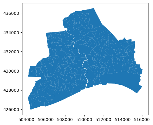
# select the LSOAs in Kingston upon Hull
gdf_lsoa_hull = gdf_lsoa_uk[gdf_lsoa_uk['LSOA21NM'].str.contains('Kingston upon Hull')]
# transfer the crs
gdf_lsoa_hull = gdf_lsoa_hull.to_crs(epsg=27700)
print(len(gdf_lsoa_hull))
gdf_lsoa_hull.plot()

168

<Axes: >

gdf_lsoa_hull.head()

	FID	LSOA21CD	LSOA21NM	LSOA21NMW	BNG_E	BNG_N	LAT	LONG	Shape__Area	Shape__Length	GlobalID	geometry
12115	12116	E01012756	Kingston upon Hull 025A		507367	430316	53.75817	-0.37294	198939.277603	3497.174098	b1f95abf-436c-4f5a-b6e1-93be9e0eb24d	POLYGON ((507433.012 430447.008, 507438.614 43...
12116	12117	E01012757	Kingston upon Hull 025B		508017	429519	53.75088	-0.36336	318088.364120	3716.172876	5f00b0d5-45c1-4529-9e08-881c4c58834d	POLYGON ((508039.325 430021.467, 508047.639 42...
12117	12118	E01012758	Kingston upon Hull 018A		507706	430320	53.75814	-0.36780	311920.300018	3772.447527	94cd85a6-b982-4038-9625-333de4b818df	POLYGON ((507791.196 430453.312, 507795.719 43...
12118	12119	E01012759	Kingston upon Hull 025C		507184	429662	53.75233	-0.37594	398184.936035	3984.903843	1516f69d-ec4e-4e2b-8f3d-81d5f680f631	POLYGON ((507088.105 429992.978, 507088.215 42...
12119	12120	E01012760	Kingston upon Hull 025D		507714	429795	53.75342	-0.36786	126002.444229	2081.849577	2e8144b1-63d2-4100-b2a5-a1fe09759513	POLYGON ((507913.848 429950.94, 507917.695 429...

# reindex
gdf_lsoa_hull.index = range(len(gdf_lsoa_hull))

# calculate the spatial weights using the Queen contiguity method
w_lsoa_hull = weights.Queen.from_dataframe(gdf_lsoa_hull, use_index='True')

# print the spatial weights as df
df_w_lsoa_hull = w_lsoa_hull.to_adjlist(drop_islands=True)
df_w_lsoa_hull

	focal	neighbor	weight
0	0	2	1.0
1	0	3	1.0
2	0	4	1.0
3	0	35	1.0
4	0	37	1.0
...	...	...	...
887	166	167	1.0
888	167	71	1.0
889	167	156	1.0
890	167	165	1.0
891	167	166	1.0

892 rows × 3 columns

Q2 solution

df_crime_hu_2024 = pd.read_csv('data/police_humberside_2024/2024-07/2024-07-humberside-street.csv')
df_crime_hu_2024

	Crime ID	Month	Reported by	Falls within	Longitude	Latitude	Location	LSOA code	LSOA name	Crime type	Last outcome category	Context
0	db0f44d9523f2ec3713b89dc85de32390d7846d4857b18...	2024-07	Humberside Police	Humberside Police	-2.268891	53.548199	On or near Rothay Close	E01004941	Bury 021A	Public order	Investigation complete; no suspect identified	NaN
1	36be51a29a5b2e9603ef61c7f0915f7a877d94082f418f...	2024-07	Humberside Police	Humberside Police	-2.290840	53.520355	On or near Venwood Road	E01005031	Bury 025A	Public order	Court result unavailable	NaN
2	1b0c316c8c3a4c0f75592f16d4672e24fc4c977eab7ae3...	2024-07	Humberside Police	Humberside Police	-1.924643	54.544159	On or near Shopping Area	E01020854	County Durham 067F	Violence and sexual offences	Unable to prosecute suspect	NaN
3	22c74bdf8fce39c14cd76207bae4fef5719cfb4658bc6f...	2024-07	Humberside Police	Humberside Police	-0.183283	51.117402	On or near Exchange Road	E01031585	Crawley 004C	Violence and sexual offences	Status update unavailable	NaN
4	b6f7155c48ca46c57cd20afcc5c6bb07a1ce1d42618415...	2024-07	Humberside Police	Humberside Police	-0.915717	53.571778	On or near Low Levels Bank	E01007559	Doncaster 008D	Vehicle crime	Investigation complete; no suspect identified	NaN
...	...	...	...	...	...	...	...	...	...	...	...	...
9105	31b720576e28ed22c8ce7d88459354c16bd69203ecc8d5...	2024-07	Humberside Police	Humberside Police	-0.786901	53.417548	On or near Southlands Drive	E01026408	West Lindsey 002F	Violence and sexual offences	Unable to prosecute suspect	NaN
9106	e03bd02394c757448d696e29eef78c95aab5d37758b808...	2024-07	Humberside Police	Humberside Police	-0.783777	53.406801	On or near Mercer Road	E01026378	West Lindsey 004A	Violence and sexual offences	Court result unavailable	NaN
9107	5eb623d7120422789578385c41c2122e7a668dfca83f0b...	2024-07	Humberside Police	Humberside Police	-0.774953	53.391906	On or near Petrol Station	E01026383	West Lindsey 004E	Violence and sexual offences	Unable to prosecute suspect	NaN
9108	61567f9efb26eac00b89587559c1c1473824198b48957a...	2024-07	Humberside Police	Humberside Police	-0.600770	53.407881	On or near Dawnhill Lane	E01026385	West Lindsey 005A	Violence and sexual offences	Unable to prosecute suspect	NaN
9109	3b6096ad0ef42e9b924002113e208a910aae54f1dcb91d...	2024-07	Humberside Police	Humberside Police	-0.563082	53.393698	On or near Creampoke Crescent	E01026386	West Lindsey 005B	Vehicle crime	Investigation complete; no suspect identified	NaN

9110 rows × 12 columns

# create the gdf from the df_crime_hu_2024 with x and y coordinates
gdf_crime_hu = gpd.GeoDataFrame(df_crime_hu_2024, geometry=gpd.points_from_xy(df_crime_hu_2024['Longitude'],
                                                                              df_crime_hu_2024['Latitude']), crs='EPSG:4326')
# transform the CRS to EPSG:27700 (British National Grid)
gdf_crime_hu = gdf_crime_hu.to_crs(epsg=27700)
gdf_crime_hu

	Crime ID	Month	Reported by	Falls within	Longitude	Latitude	Location	LSOA code	LSOA name	Crime type	Last outcome category	Context	geometry
0	db0f44d9523f2ec3713b89dc85de32390d7846d4857b18...	2024-07	Humberside Police	Humberside Police	-2.268891	53.548199	On or near Rothay Close	E01004941	Bury 021A	Public order	Investigation complete; no suspect identified	NaN	POINT (382280.834 405761.213)
1	36be51a29a5b2e9603ef61c7f0915f7a877d94082f418f...	2024-07	Humberside Police	Humberside Police	-2.290840	53.520355	On or near Venwood Road	E01005031	Bury 025A	Public order	Court result unavailable	NaN	POINT (380813.893 402669.101)
2	1b0c316c8c3a4c0f75592f16d4672e24fc4c977eab7ae3...	2024-07	Humberside Police	Humberside Police	-1.924643	54.544159	On or near Shopping Area	E01020854	County Durham 067F	Violence and sexual offences	Unable to prosecute suspect	NaN	POINT (404973.562 516546.025)
3	22c74bdf8fce39c14cd76207bae4fef5719cfb4658bc6f...	2024-07	Humberside Police	Humberside Police	-0.183283	51.117402	On or near Exchange Road	E01031585	Crawley 004C	Violence and sexual offences	Status update unavailable	NaN	POINT (527250.11 136915.397)
4	b6f7155c48ca46c57cd20afcc5c6bb07a1ce1d42618415...	2024-07	Humberside Police	Humberside Police	-0.915717	53.571778	On or near Low Levels Bank	E01007559	Doncaster 008D	Vehicle crime	Investigation complete; no suspect identified	NaN	POINT (471900.336 408896.718)
...	...	...	...	...	...	...	...	...	...	...	...	...	...
9105	31b720576e28ed22c8ce7d88459354c16bd69203ecc8d5...	2024-07	Humberside Police	Humberside Police	-0.786901	53.417548	On or near Southlands Drive	E01026408	West Lindsey 002F	Violence and sexual offences	Unable to prosecute suspect	NaN	POINT (480722.247 391876.638)
9106	e03bd02394c757448d696e29eef78c95aab5d37758b808...	2024-07	Humberside Police	Humberside Police	-0.783777	53.406801	On or near Mercer Road	E01026378	West Lindsey 004A	Violence and sexual offences	Court result unavailable	NaN	POINT (480950.184 390684.609)
9107	5eb623d7120422789578385c41c2122e7a668dfca83f0b...	2024-07	Humberside Police	Humberside Police	-0.774953	53.391906	On or near Petrol Station	E01026383	West Lindsey 004E	Violence and sexual offences	Unable to prosecute suspect	NaN	POINT (481565.151 389037.635)
9108	61567f9efb26eac00b89587559c1c1473824198b48957a...	2024-07	Humberside Police	Humberside Police	-0.600770	53.407881	On or near Dawnhill Lane	E01026385	West Lindsey 005A	Violence and sexual offences	Unable to prosecute suspect	NaN	POINT (493113.206 391027.523)
9109	3b6096ad0ef42e9b924002113e208a910aae54f1dcb91d...	2024-07	Humberside Police	Humberside Police	-0.563082	53.393698	On or near Creampoke Crescent	E01026386	West Lindsey 005B	Vehicle crime	Investigation complete; no suspect identified	NaN	POINT (495650.172 389499.55)

9110 rows × 13 columns

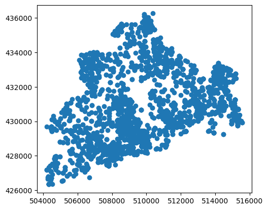
# spatial join the gdf_crime_hu and gdf_lsoa_hull to get the LSOA index for each crime incident (we don't use the 'LSOA codes' in the df_crime_hu_2024)
gdf_crime_hu_lsoa = gpd.sjoin(gdf_crime_hu, gdf_lsoa_hull, how='inner', predicate='within')
gdf_crime_hu_lsoa

	Crime ID	Month	Reported by	Falls within	Longitude	Latitude	Location	LSOA code	LSOA name	Crime type	...	LSOA21CD	LSOA21NM	LSOA21NMW	BNG_E	BNG_N	LAT	LONG	Shape__Area	Shape__Length	GlobalID
2194	NaN	2024-07	Humberside Police	Humberside Police	-0.319102	53.795305	On or near Finningley Garth	E01012782	Kingston upon Hull 002A	Anti-social behaviour	...	E01012782	Kingston upon Hull 002A		510564	434676	53.79667	-0.32291	295014.267838	2717.829437	4bac5250-9916-4da1-87ac-00c02f2d47b4
2195	2914efb412b1e124dc12b379fe395d457d11b998690d24...	2024-07	Humberside Police	Humberside Police	-0.325162	53.797160	On or near Abingdon Garth	E01012782	Kingston upon Hull 002A	Bicycle theft	...	E01012782	Kingston upon Hull 002A		510564	434676	53.79667	-0.32291	295014.267838	2717.829437	4bac5250-9916-4da1-87ac-00c02f2d47b4
2196	f8c053aed0021740e7e17f577414c52eff339a3fe85a80...	2024-07	Humberside Police	Humberside Police	-0.320579	53.796719	On or near Digby Garth	E01012782	Kingston upon Hull 002A	Burglary	...	E01012782	Kingston upon Hull 002A		510564	434676	53.79667	-0.32291	295014.267838	2717.829437	4bac5250-9916-4da1-87ac-00c02f2d47b4
2197	70598a4effd9969de667c33037522cd7d3209c03b8e308...	2024-07	Humberside Police	Humberside Police	-0.325162	53.797160	On or near Abingdon Garth	E01012782	Kingston upon Hull 002A	Criminal damage and arson	...	E01012782	Kingston upon Hull 002A		510564	434676	53.79667	-0.32291	295014.267838	2717.829437	4bac5250-9916-4da1-87ac-00c02f2d47b4
2198	f6632e2e3eed766b50dd277da0aa143e0fec44abbbf554...	2024-07	Humberside Police	Humberside Police	-0.325162	53.797160	On or near Abingdon Garth	E01012782	Kingston upon Hull 002A	Other theft	...	E01012782	Kingston upon Hull 002A		510564	434676	53.79667	-0.32291	295014.267838	2717.829437	4bac5250-9916-4da1-87ac-00c02f2d47b4
...	...	...	...	...	...	...	...	...	...	...	...	...	...	...	...	...	...	...	...	...	...
5650	a43df72a23c5e5fc6944c3769ed323317c1879693b6571...	2024-07	Humberside Police	Humberside Police	-0.347889	53.795045	On or near Shopping Area	E01033105	Kingston upon Hull 035D	Other crime	...	E01033105	Kingston upon Hull 035D		509270	434654	53.79675	-0.34256	407379.168350	3953.907070	d4f9f0ce-a99e-47be-995b-5af0f302b061
5651	1f5ce2f185ded208a8e75f9a6a79de96007917d15fb824...	2024-07	Humberside Police	Humberside Police	-0.355095	53.793485	On or near Raich Carter Way	E01033107	Kingston upon Hull 035E	Bicycle theft	...	E01033107	Kingston upon Hull 035E		508618	434547	53.79592	-0.35249	392191.723434	3331.231133	f698240e-05d9-4a6a-8c12-ba6f537ddef1
5652	37172c13e7e745ddd24c1e82f94205856c60dba94be169...	2024-07	Humberside Police	Humberside Police	-0.355095	53.793485	On or near Raich Carter Way	E01033107	Kingston upon Hull 035E	Bicycle theft	...	E01033107	Kingston upon Hull 035E		508618	434547	53.79592	-0.35249	392191.723434	3331.231133	f698240e-05d9-4a6a-8c12-ba6f537ddef1
5653	556d2c014b63fedb8ce14666a9700113625ad882f95a90...	2024-07	Humberside Police	Humberside Police	-0.348154	53.798576	On or near Halecroft Park	E01033107	Kingston upon Hull 035E	Violence and sexual offences	...	E01033107	Kingston upon Hull 035E		508618	434547	53.79592	-0.35249	392191.723434	3331.231133	f698240e-05d9-4a6a-8c12-ba6f537ddef1
5654	4a15b8fdf636482baa1bb829c9fcc08cf76b5cc9f2e323...	2024-07	Humberside Police	Humberside Police	-0.350433	53.795452	On or near Runnymede Way	E01033107	Kingston upon Hull 035E	Other crime	...	E01033107	Kingston upon Hull 035E		508618	434547	53.79592	-0.35249	392191.723434	3331.231133	f698240e-05d9-4a6a-8c12-ba6f537ddef1

3461 rows × 25 columns

gdf_crime_hu_lsoa.plot()

<Axes: >

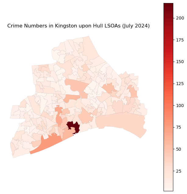
df_crime_hull_agg = gdf_crime_hu_lsoa.groupby(['LSOA21CD', 'Month']).agg({'Crime ID': 'count'}).reset_index().rename(columns={'Crime ID': 'Numbers'})
df_crime_hull_agg

	LSOA21CD	Month	Numbers
0	E01012756	2024-07	13
1	E01012757	2024-07	20
2	E01012758	2024-07	6
3	E01012759	2024-07	31
4	E01012760	2024-07	7
...	...	...	...
163	E01035468	2024-07	10
164	E01035469	2024-07	6
165	E01035470	2024-07	12
166	E01035471	2024-07	9
167	E01035472	2024-07	4

168 rows × 3 columns

# set the geometry to the df_crime_hull_agg
gdf_crime_hull_agg = pd.merge(gdf_lsoa_hull, df_crime_hull_agg, on='LSOA21CD', how='left')

fig, ax = plt.subplots(figsize=(8, 8))
# plot the crime data
gdf_crime_hull_agg.plot(ax=ax, column='Numbers', cmap='Reds', edgecolor='black', linewidth=0.05, legend=True)
ax.set_title('Crime Numbers in Kingston upon Hull LSOAs (July 2024)')
ax.axis('off')
plt.show()

Q3 solution

# caculate the global moran's I
moran = esda.Moran(gdf_crime_hull_agg['Numbers'].values, w_lsoa_hull)
print(moran.I, moran.p_sim)

0.2315067482911263 0.001

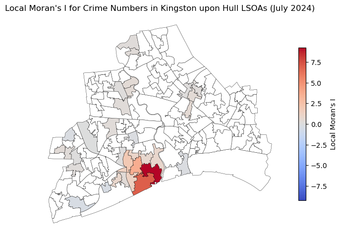
Q4 solution

# compute the local moran's I for the crime data
local_moran = esda.Moran_Local(gdf_crime_hull_agg['Numbers'].values, w_lsoa_hull)
# plot the local moran's I
gdf_crime_hull_agg['local_moran'] = local_moran.Is
gdf_crime_hull_agg['local_moran_p'] = local_moran.p_sim
fig, ax = plt.subplots(figsize=(8, 8))
gdf_crime_hull_agg[gdf_crime_hull_agg['local_moran_p'] < 0.05].plot(ax=ax, column='local_moran',
                                                                    cmap='coolwarm', edgecolor='black',
                                                                    linewidth=0.3, legend=True,
                                                                    vmin=-max(local_moran.Is), vmax=max(local_moran.Is),
                                                                    legend_kwds={'shrink': 0.5, 'orientation': 'vertical', 'label': 'Local Moran\'s I'})
# plot the not significant areas
gdf_crime_hull_agg[gdf_crime_hull_agg['local_moran_p'] >= 0.05].plot(ax=ax, color='white', edgecolor='black', linewidth=0.3)
ax.set_title('Local Moran\'s I for Crime Numbers in Kingston upon Hull LSOAs (July 2024)')
ax.axis('off')

(503532.6564838799, 516643.2624241113, 425425.5469577427, 437061.9176401592)

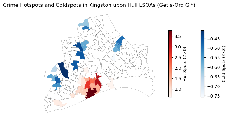
# compute the Getis-Ord Gi* for the crime data
gi = esda.G_Local(gdf_crime_hull_agg['Numbers'].values, w_lsoa_hull)
# add the Getis-Ord Gi* to the gdf_crime_hull_agg
gdf_crime_hull_agg['gi'] = gi.Zs
gdf_crime_hull_agg['gi_p'] = gi.p_sim

# Create a figure and axis
fig, ax = plt.subplots(figsize=(8, 8))

# Plot not significant areas (p_sim >= 0.05)  
gdf_crime_hull_agg[gdf_crime_hull_agg['gi_p'] >= 0.05].plot(
    ax=ax, color='white', edgecolor='black', linewidth=0.15)

# Plot cold spots (negative Z-scores and p_sim < 0.05)
gdf_crime_hull_agg[(gdf_crime_hull_agg['gi'] < 0) & (gdf_crime_hull_agg['gi_p'] < 0.05)].plot(
    column='gi',
    ax=ax,
    cmap='Blues',
    legend=True,
    legend_kwds={'shrink': 0.35, 'orientation': 'vertical', 'label': 'Cold Spots (Z<0)'},
    linewidth=0.15)

# Plot hot spots (positive Z-scores and p_sim < 0.05)  
gdf_crime_hull_agg[(gdf_crime_hull_agg['gi'] > 0) & (gdf_crime_hull_agg['gi_p'] < 0.05)].plot(
    column='gi',
    ax=ax,
    cmap='Reds',
    legend=True,
    legend_kwds={'shrink': 0.35, 'orientation': 'vertical', 'label': 'Hot Spots (Z>0)'},
    linewidth=0.15)

ax.axis('off')
plt.title('Crime Hotspots and Coldspots in Kingston upon Hull LSOAs (Getis-Ord Gi*)')
plt.show()