Week8 Lab Tutorial Timeline
Time |
Activity |
|---|---|
16:00–16:05 |
Introduction — Overview of the main tasks for the lab tutorials |
16:05–16:45 |
Tutorial: Machine learning for spatio-temporal analysis — Follow Section 8.1-8.2 of the Jupyter Notebook to practice the SVM, CV and spatial SV framework |
16:45–17:30 |
Tutorial: Machine learning for spatio-temporal analysis — Follow Section 8.3 of the Jupyter Notebook to practice the RF |
17:30–17:55 |
Quiz — Complete quiz tasks |
17:55–18:00 |
Wrap-up — Recap key points and address final questions |
For this module’s lab tutorials, you can download all the required data using the provided link (click).
Please make sure that both the Jupyter Notebook file and the data and img folder are placed in the same directory (specifically within the STBDA_lab folder) to ensure the code runs correctly.
Week 8 Key Takeaways:
Understand the fundamentals of machine learning (ML) in space and time, including the ML workflow and tasks in spatial and spatio-temporal prediction.
Learn about spatial cross-validation (CV) and its importance in avoiding data leakage in spatial data.
Implement a Support Vector Machine (SVM) regression model for spatial prediction, including hyperparameter tuning using Random CV.
Evaluate the trained SVM model using both Random CV and spatial CV, and understand the differences in performance.
Explore the use of Random Forests (RF) for spatial and temporal prediction tasks.
8 Machine learning for spatio-temporal analysis 1#
8.1 Fundamentals of ML in space and time#
8.1.1 Machine learning (ML) workflow#
Machine learning (ML) is a branch of artificial intelligence that focuses on developing algorithms and models that enable computers to learn and make predictions from data without being explicitly programmed. Key steps in one typical supervised ML workflow:
Problem Definition: define the objective (e.g., classification or regression).
Data Collection: gather data from relevant sources (\(X\) features/predictors/independent variables and \(y\) labels/targets/responses/dependent variables).
Initial Data Preprocessing: handle missing values, remove duplicates, encode categorical variables (if necessary), outlier handling (if necessary).
Data Splitting: split the dataset into training, validation, and test sets (e.g., 70/15/15 or 80/20 rule).
Feature Scaling: (Normalization/Standardization), Fit the scaler on the training set and test sets.
Further Preprocessing : feature selection, dimensionality reduction (e.g., PCA) fit only on training data if necessary.
Model Training and Hyperparameter Tuning (Cross-Validation): Train the model using the training set and optimise the model using Hyperparameter Tuning (grid search, random search, or Bayesian optimization) –> performance metrics on the training set.
Model Evaluation and testing: evaluate on the validation/test set –> performance metrics on the testing set.
Deployment: deploy the trained model into a production environment.
8.1.2 ML tasks in space and time#
1.Spatial prediction – Space (X, Y):
Spatial prediction focuses only on predicting values at unobserved spatial units/locations using data from known units/locations (under the same observation time/ no time factor).
Example: Assume there are 100 neighborhoods in a city. You have house price data for 90 of these neighborhoods for the year 2024. However, for the remaining 10 neighborhoods, no house price data is available — possibly because no houses were sold in those areas during that year. Your goal is to predict house prices in those 10 neighborhoods based solely on the spatial patterns learned from the 90 neighborhoods with other spatial available data (No historical (temporal) data is considered).
2.Spatial-temporal prediction – Space (X, Y) + Time (T):
Spatial-temporal prediction considers both space and time dynamics, which are aiming to predict values at spatial units for a specific time, i.e., to answer how things change over time and across space.
Example: Assume there are 100 neighborhoods in a city. You have house price data for all of these neighborhoods for the year 2013–2023. Your goal is to predict house prices for those 100 neighborhoods in 2024 based on the historical house price data (with other available data).
8.1.3 Spatial cross-validation (CV)#
Spatial cross-validation (CV) is a validation technique designed specifically for spatial data. It aims to avoid data leakage and produce realistic performance estimates by accounting for spatial autocorrelation (i.e., nearby locations tend to have similar values).
Why we need spatial CV: Random CV assumes data points are independent and identically distributed, but in spatial data, nearby observations are often similar (spatial autocorrelation), so if train and test sets are spatially close, the model may look like it performs well — but it’s just memorizing nearby areas.
Spatial CV methods include( Ref link ):
Method |
Description |
Use Cases |
|---|---|---|
1. Clustering-Based Spatial CV |
Spatial units (e.g., areas or points) are grouped using clustering (e.g., KMeans) |
Heterogeneous areas, no clear spatial boundaries |
2. Grid-Based Spatial CV |
Study area is divided into uniform grid cells (e.g., 5km × 5km blocks), and CV is done across cells |
Raster data, environmental monitoring, spatial interpolation |
3. Geo-Attribute-Based CV |
Spatial units grouped based on spatial and non-spatial features (e.g., census area, adminstrative area, city, region) |
Urban modeling, socio-spatial segregation, enriched context |
4. Spatial Leave-One-Out CV |
Each spatial unit is left out in turn; training excludes that unit and often a buffer zone around it |
Small datasets or models needing strict leakage control |
8.2 Spatial prediction using Support Vector Machine (SVM)#
8.2.1 SVM regression model and hyperpramer using GridSearch + Random CV#
Support Vector Machine (SVM) is a supervised machine learning algorithm used for classification and regression problems. The core idea of SVM is to find the optimal hyperplane that separates different classes in the feature space with the maximum margin. For non-linearly separable data, SVM uses kernel functions to project the data into a higher-dimensional space where a linear separator is possible.
Key concepts:
Margin: The distance between the hyperplane and the nearest data points from each class (support vectors).
Support Vectors: Data points that lie closest to the decision boundary and influence its position.
Kernel Trick: A technique to transform data into higher dimensions using functions like polynomial, radial basis function (RBF), etc.
The important parameters in SVM from the sklearn library:
kernel(str): Specifies the kernel type to be used:linearpoly(polynomial)rbf(radial basis function, default)sigmoid
C(float): Regularization parameter. A smaller C encourages a wider margin (more tolerance to misclassification), while a larger C aims for accurate classification (less tolerance).gamma(float or scale / auto ): Kernel coefficient for ‘rbf’, ‘poly’, and ‘sigmoid’.scale(default): 1 / (n_features * X.var())auto: 1 / n_featuresFloat: custom value
degree(int): Degree of the polynomial kernel function (‘poly’). Ignored by other kernels.coef0(float): Independent term in kernel function. It’s significant in ‘poly’ and ‘sigmoid’.shrinking(bool): Whether to use the shrinking heuristic, which can speed up training.decision_function_shape(str): One-vs-one (‘ovo’) or one-vs-rest (‘ovr’). Default is ‘ovr’.epsilon: Epsilon in the epsilon-SVR model. Specifies the epsilon-tube within which no penalty is associated in the training loss function.
# Import necessary libraries
import geopandas as gpd
import pandas as pd
import matplotlib.pyplot as plt
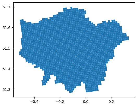
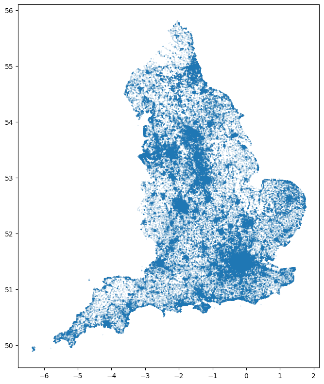
We use the UK open police data in London to demonstrate the machine learning for a spatial prediction task. Apart from the spatial unit of analysis – LSOA previously, we use a different geospatial unit data called GEOSTAT 1km grid from ONS add important place data – Point of Interest data from OpenStreetMap as the feature data resources. A point of interest (POI) is a specific location or place (like restaurants, cafes, bars and hospitals) that is of particular significance or utility within a geographic context.
Step 1 Problem definition:
We will use the POI data (X features) to predict the crime levels (y targets) across London grids (1km and 1km) via the machine learning models.
Step 2 data collection and preprocessing:
# Load the house price data
gdf_grid = gpd.read_file('data/GEOSTAT_Dec_2011_GEC_in_the_United_Kingdom_2022.geojson')
gdf_grid.head()
| OBJECTID | grd_fixid | grd_floaid | grd_newid | pcd_count | tot_p | tot_m | tot_f | tot_hh | GlobalID | geometry | |
|---|---|---|---|---|---|---|---|---|---|---|---|
| 0 | 1 | 4.0.31510000.31050000 | 3151.3105.4 | 1kmN3105E3151 | 0 | 0 | 0 | 0 | 0 | c142c42b-5160-4760-a836-956a3920caf8 | POLYGON ((-6.41829 49.87519, -6.41852 49.87527... |
| 1 | 2 | 4.0.31520000.31040000 | 3152.3104.4 | 1kmN3104E3152 | 0 | 0 | 0 | 0 | 0 | 26709ad2-2ae8-4f76-95f4-850c60e9c8e6 | POLYGON ((-6.41461 49.87373, -6.40491 49.87515... |
| 2 | 3 | 4.0.31520000.31050000 | 3152.3105.4 | 1kmN3105E3152 | 0 | 0 | 0 | 0 | 0 | e477a513-48a2-4012-9cd7-3063ac2bc6c6 | POLYGON ((-6.40698 49.8838, -6.40414 49.87568,... |
| 3 | 4 | 4.0.31520000.31060000 | 3152.3106.4 | 1kmN3106E3152 | 0 | 0 | 0 | 0 | 0 | 8d1562d5-3252-40ef-858e-c80391bebefe | POLYGON ((-6.40726 49.88398, -6.42047 49.88204... |
| 4 | 5 | 4.0.31530000.31050000 | 3153.3105.4 | 1kmN3105E3153 | 0 | 0 | 0 | 0 | 0 | 2952357c-da71-4e17-93a0-ace5e73e86d4 | POLYGON ((-6.40414 49.87568, -6.40698 49.8838,... |
# There are 260661 grids (1km * 1km) in the UK
print(len(gdf_grid))
260661
# read the London boundary
gdf_london_bound = gpd.read_file('data/whole_london_boundary.geojson')
# to select the Grids in London, we do not use the overlay to clip the shap but use the spatial join to select the grids of London
gdf_london_grid = gpd.sjoin(gdf_grid, gdf_london_bound, how='inner', predicate='intersects')
# There are 1733 grids of London
gdf_london_grid
| OBJECTID | grd_fixid | grd_floaid | grd_newid | pcd_count | tot_p | tot_m | tot_f | tot_hh | GlobalID | geometry | index_right | name | |
|---|---|---|---|---|---|---|---|---|---|---|---|---|---|
| 214288 | 214289 | 4.0.35930000.32030000 | 3593.3203.4 | 1kmN3203E3593 | 3 | 9 | 5 | 4 | 5 | 9f0c1e1f-e8fa-40ca-a969-d1aedbefa750 | POLYGON ((-0.50339 51.46588, -0.51765 51.46459... | 0 | Greater London |
| 214289 | 214290 | 4.0.35930000.32040000 | 3593.3204.4 | 1kmN3204E3593 | 54 | 1957 | 1029 | 928 | 833 | e2530627-9630-4200-ae13-788341456d76 | POLYGON ((-0.50545 51.47476, -0.51972 51.47347... | 0 | Greater London |
| 214864 | 214865 | 4.0.35940000.32020000 | 3594.3202.4 | 1kmN3202E3594 | 13 | 445 | 223 | 222 | 169 | bf801f98-5376-4c37-8bcb-d80ae9af1f0b | POLYGON ((-0.48707 51.45829, -0.50133 51.457, ... | 0 | Greater London |
| 214865 | 214866 | 4.0.35940000.32030000 | 3594.3203.4 | 1kmN3203E3594 | 3 | 34 | 18 | 16 | 11 | 472a8640-40e0-4c94-8eb5-37647847dc99 | POLYGON ((-0.48913 51.46717, -0.50339 51.46588... | 0 | Greater London |
| 214866 | 214867 | 4.0.35940000.32040000 | 3594.3204.4 | 1kmN3204E3594 | 1 | 15 | 9 | 6 | 8 | c21982c0-0d13-43df-8fa5-f77c28fba3d6 | POLYGON ((-0.49118 51.47605, -0.50545 51.47476... | 0 | Greater London |
| ... | ... | ... | ... | ... | ... | ... | ... | ... | ... | ... | ... | ... | ... |
| 240547 | 240548 | 4.0.36510000.32040000 | 3651.3204.4 | 1kmN3204E3651 | 0 | 0 | 0 | 0 | 0 | c1be8f1c-6c91-4dca-aad2-ce9f51538b0e | POLYGON ((0.32328 51.54665, 0.30897 51.54546, ... | 0 | Greater London |
| 240548 | 240549 | 4.0.36510000.32050000 | 3651.3205.4 | 1kmN3205E3651 | 2 | 73 | 41 | 32 | 25 | 65336bd5-772b-4398-a0de-4ccb1b438479 | POLYGON ((0.32137 51.55555, 0.30706 51.55436, ... | 0 | Greater London |
| 240549 | 240550 | 4.0.36510000.32060000 | 3651.3206.4 | 1kmN3206E3651 | 2 | 36 | 16 | 20 | 13 | befe6e14-0fef-4c44-8440-c3e80c139c63 | POLYGON ((0.31947 51.56445, 0.30515 51.56326, ... | 0 | Greater London |
| 240928 | 240929 | 4.0.36520000.32030000 | 3652.3203.4 | 1kmN3203E3652 | 2 | 26 | 15 | 11 | 12 | 96832cf0-62a9-49a4-b442-ac283b90db87 | POLYGON ((0.33949 51.53894, 0.32518 51.53776, ... | 0 | Greater London |
| 240929 | 240930 | 4.0.36520000.32040000 | 3652.3204.4 | 1kmN3204E3652 | 0 | 0 | 0 | 0 | 0 | f0c429cf-e001-432e-a41b-259a3c9e6582 | POLYGON ((0.33759 51.54784, 0.32328 51.54665, ... | 0 | Greater London |
1733 rows × 13 columns
# drop the index_right column
gdf_london_grid = gdf_london_grid.drop(columns=['index_right'])
# plot the London grid data
gdf_london_grid.plot(figsize= (6,6))
<Axes: >
# here we only use the gis_osm_pois_free_1.shp file
gdf_poi = gpd.read_file('data/osm_england-latest-free-shp/gis_osm_pois_free_1.shp')
gdf_poi.columns
Index(['osm_id', 'code', 'fclass', 'name', 'geometry'], dtype='object')
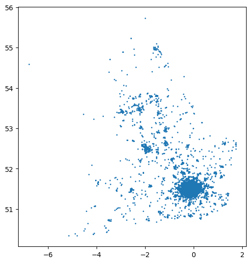
gdf_poi.plot(markersize=0.01, figsize=(8,12))
<Axes: >
# spatila join the poi data with the grid data
gdf_poi_grid = gpd.sjoin(gdf_poi, gdf_london_grid, how='left', predicate='intersects')
gdf_poi_grid_s = gdf_poi_grid[~gdf_poi_grid.grd_newid.isna()]
# we calculate the numbers and poi type for each grid
df_poi_counts = gdf_poi_grid_s.groupby(['grd_newid']).size().reset_index(name='poi_counts')
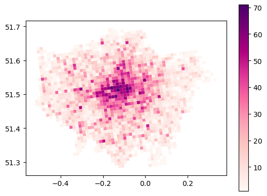
df_poi_types = gdf_poi_grid_s.groupby(['grd_newid']).nunique()['fclass'].reset_index(name='poi_types')
# merge the poi data with the grid data one by one
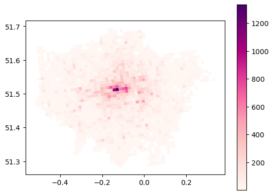
gdf_london_grid_poi = gdf_london_grid.merge(df_poi_counts, on='grd_newid', how='left')
gdf_poi_grid_s_poi_type = gdf_london_grid_poi.merge(df_poi_types, on='grd_newid', how='left')
gdf_poi_grid_s_poi_type
| OBJECTID | grd_fixid | grd_floaid | grd_newid | pcd_count | tot_p | tot_m | tot_f | tot_hh | GlobalID | geometry | name | poi_counts | poi_types | |
|---|---|---|---|---|---|---|---|---|---|---|---|---|---|---|
| 0 | 214289 | 4.0.35930000.32030000 | 3593.3203.4 | 1kmN3203E3593 | 3 | 9 | 5 | 4 | 5 | 9f0c1e1f-e8fa-40ca-a969-d1aedbefa750 | POLYGON ((-0.50339 51.46588, -0.51765 51.46459... | Greater London | 3.0 | 3.0 |
| 1 | 214290 | 4.0.35930000.32040000 | 3593.3204.4 | 1kmN3204E3593 | 54 | 1957 | 1029 | 928 | 833 | e2530627-9630-4200-ae13-788341456d76 | POLYGON ((-0.50545 51.47476, -0.51972 51.47347... | Greater London | 5.0 | 5.0 |
| 2 | 214865 | 4.0.35940000.32020000 | 3594.3202.4 | 1kmN3202E3594 | 13 | 445 | 223 | 222 | 169 | bf801f98-5376-4c37-8bcb-d80ae9af1f0b | POLYGON ((-0.48707 51.45829, -0.50133 51.457, ... | Greater London | 1.0 | 1.0 |
| 3 | 214866 | 4.0.35940000.32030000 | 3594.3203.4 | 1kmN3203E3594 | 3 | 34 | 18 | 16 | 11 | 472a8640-40e0-4c94-8eb5-37647847dc99 | POLYGON ((-0.48913 51.46717, -0.50339 51.46588... | Greater London | 8.0 | 4.0 |
| 4 | 214867 | 4.0.35940000.32040000 | 3594.3204.4 | 1kmN3204E3594 | 1 | 15 | 9 | 6 | 8 | c21982c0-0d13-43df-8fa5-f77c28fba3d6 | POLYGON ((-0.49118 51.47605, -0.50545 51.47476... | Greater London | 2.0 | 1.0 |
| ... | ... | ... | ... | ... | ... | ... | ... | ... | ... | ... | ... | ... | ... | ... |
| 1728 | 240548 | 4.0.36510000.32040000 | 3651.3204.4 | 1kmN3204E3651 | 0 | 0 | 0 | 0 | 0 | c1be8f1c-6c91-4dca-aad2-ce9f51538b0e | POLYGON ((0.32328 51.54665, 0.30897 51.54546, ... | Greater London | NaN | NaN |
| 1729 | 240549 | 4.0.36510000.32050000 | 3651.3205.4 | 1kmN3205E3651 | 2 | 73 | 41 | 32 | 25 | 65336bd5-772b-4398-a0de-4ccb1b438479 | POLYGON ((0.32137 51.55555, 0.30706 51.55436, ... | Greater London | 2.0 | 2.0 |
| 1730 | 240550 | 4.0.36510000.32060000 | 3651.3206.4 | 1kmN3206E3651 | 2 | 36 | 16 | 20 | 13 | befe6e14-0fef-4c44-8440-c3e80c139c63 | POLYGON ((0.31947 51.56445, 0.30515 51.56326, ... | Greater London | NaN | NaN |
| 1731 | 240929 | 4.0.36520000.32030000 | 3652.3203.4 | 1kmN3203E3652 | 2 | 26 | 15 | 11 | 12 | 96832cf0-62a9-49a4-b442-ac283b90db87 | POLYGON ((0.33949 51.53894, 0.32518 51.53776, ... | Greater London | 1.0 | 1.0 |
| 1732 | 240930 | 4.0.36520000.32040000 | 3652.3204.4 | 1kmN3204E3652 | 0 | 0 | 0 | 0 | 0 | f0c429cf-e001-432e-a41b-259a3c9e6582 | POLYGON ((0.33759 51.54784, 0.32328 51.54665, ... | Greater London | NaN | NaN |
1733 rows × 14 columns
gdf_poi_grid_s_poi_type.plot(column='poi_counts', cmap='RdPu', legend=True)
<Axes: >
gdf_poi_grid_s_poi_type.plot(column='poi_types', cmap='RdPu', legend=True)
<Axes: >
# read the crime data all in police_met_city_2024/2024-0*/**.csv
import glob
# Get all CSV files in the directory
csv_files = glob.glob('data/police_met_city_2024/2024-**/**/*.csv', recursive=True)
# Read and concatenate all CSV files into a single DataFrame
df_crime = pd.concat((pd.read_csv(file) for file in csv_files), ignore_index=True)
# create a GeoDataFrame from the crime data
import geopandas as gpd
gdf_crime = gpd.GeoDataFrame(df_crime, geometry=gpd.points_from_xy(df_crime['Longitude'], df_crime['Latitude']), crs='EPSG:4326')
gdf_crime
| Crime ID | Month | Reported by | Falls within | Longitude | Latitude | Location | LSOA code | LSOA name | Crime type | Last outcome category | Context | geometry | |
|---|---|---|---|---|---|---|---|---|---|---|---|---|---|
| 0 | b74d06161e2425ef2abf28345aa962fa862753669659d3... | 2024-09 | City of London Police | City of London Police | -0.107682 | 51.517786 | On or near B521 | E01000917 | Camden 027C | Robbery | Unable to prosecute suspect | NaN | POINT (-0.10768 51.51779) |
| 1 | ab9f963604d03486ffbefec80f9f9296c7f65ecd4cd047... | 2024-09 | City of London Police | City of London Police | -0.107682 | 51.517786 | On or near B521 | E01000917 | Camden 027C | Violence and sexual offences | Unable to prosecute suspect | NaN | POINT (-0.10768 51.51779) |
| 2 | 7eaad3255f757cf5073dfd3712193f4497e788b3f6519f... | 2024-09 | City of London Police | City of London Police | -0.112096 | 51.515942 | On or near Nightclub | E01000914 | Camden 028B | Violence and sexual offences | Status update unavailable | NaN | POINT (-0.1121 51.51594) |
| 3 | 71c1e6edfb73383e82ca6acdc1c9c0ef015334b529f298... | 2024-09 | City of London Police | City of London Police | -0.111596 | 51.518281 | On or near Chancery Lane | E01000914 | Camden 028B | Violence and sexual offences | Status update unavailable | NaN | POINT (-0.1116 51.51828) |
| 4 | 06e7c6b6541166a8abe71de2593b9576c5e26215e349e4... | 2024-09 | City of London Police | City of London Police | -0.098519 | 51.517332 | On or near Little Britain | E01000001 | City of London 001A | Other theft | Investigation complete; no suspect identified | NaN | POINT (-0.09852 51.51733) |
| ... | ... | ... | ... | ... | ... | ... | ... | ... | ... | ... | ... | ... | ... |
| 1149316 | 255e00edd07e15d153995d97bfcb22dc9b43055f10fafe... | 2024-10 | Metropolitan Police Service | Metropolitan Police Service | -2.059862 | 52.604816 | On or near Stubby Lane | E01010563 | Wolverhampton 010D | Violence and sexual offences | Status update unavailable | NaN | POINT (-2.05986 52.60482) |
| 1149317 | ada15de8fd97cc0d01e54aa33cc54b1327e38a3b012514... | 2024-10 | Metropolitan Police Service | Metropolitan Police Service | -2.132925 | 52.585743 | On or near Clarence Street | E01034312 | Wolverhampton 020G | Violence and sexual offences | Status update unavailable | NaN | POINT (-2.13292 52.58574) |
| 1149318 | 820ad95840e882e48b74938cb919e05df6b5321d3abce9... | 2024-10 | Metropolitan Police Service | Metropolitan Police Service | -2.123708 | 52.583362 | On or near Old Hall Street | E01034313 | Wolverhampton 020H | Other theft | Status update unavailable | NaN | POINT (-2.12371 52.58336) |
| 1149319 | fdd17e2c1eff3d47060559feaa3f4e9259dbf13e1088e2... | 2024-10 | Metropolitan Police Service | Metropolitan Police Service | -2.095217 | 52.566487 | On or near Detling Drive | E01010450 | Wolverhampton 029B | Other crime | Status update unavailable | NaN | POINT (-2.09522 52.56649) |
| 1149320 | bb019d86db42a192000d2c99522ce53a4e2f5e4a364a34... | 2024-10 | Metropolitan Police Service | Metropolitan Police Service | -2.182265 | 52.225795 | On or near Sling Lane | E01032400 | Wychavon 006B | Violence and sexual offences | Status update unavailable | NaN | POINT (-2.18226 52.2258) |
1149321 rows × 13 columns
gdf_crime.plot(markersize=1, figsize=(6,8))
<Axes: >
# spatial join the crime data with the grid data
gdf_crime_grid = gpd.sjoin(gdf_crime, gdf_london_grid_poi, how='left', predicate='intersects')
# gropby the grid id, month and count the number of all crime types
df_crime = gdf_crime_grid.groupby(['grd_newid', 'Month']).size().reset_index(name='crime_counts')
df_crime
| grd_newid | Month | crime_counts | |
|---|---|---|---|
| 0 | 1kmN3178E3627 | 2024-07 | 1 |
| 1 | 1kmN3178E3628 | 2024-11 | 1 |
| 2 | 1kmN3178E3629 | 2024-09 | 1 |
| 3 | 1kmN3178E3630 | 2024-11 | 1 |
| 4 | 1kmN3179E3617 | 2024-10 | 1 |
| ... | ... | ... | ... |
| 17989 | 1kmN3223E3625 | 2024-11 | 2 |
| 17990 | 1kmN3224E3620 | 2024-03 | 1 |
| 17991 | 1kmN3224E3620 | 2024-05 | 1 |
| 17992 | 1kmN3224E3620 | 2024-07 | 1 |
| 17993 | 1kmN3224E3620 | 2024-11 | 1 |
17994 rows × 3 columns
# reshape the df_crime to have a column for each month
df_crime_pivot = df_crime.pivot(index='grd_newid', columns='Month', values='crime_counts').fillna(0)
df_crime_pivot
| Month | 2024-01 | 2024-02 | 2024-03 | 2024-04 | 2024-05 | 2024-06 | 2024-07 | 2024-08 | 2024-09 | 2024-10 | 2024-11 | 2024-12 |
|---|---|---|---|---|---|---|---|---|---|---|---|---|
| grd_newid | ||||||||||||
| 1kmN3178E3627 | 0.0 | 0.0 | 0.0 | 0.0 | 0.0 | 0.0 | 1.0 | 0.0 | 0.0 | 0.0 | 0.0 | 0.0 |
| 1kmN3178E3628 | 0.0 | 0.0 | 0.0 | 0.0 | 0.0 | 0.0 | 0.0 | 0.0 | 0.0 | 0.0 | 1.0 | 0.0 |
| 1kmN3178E3629 | 0.0 | 0.0 | 0.0 | 0.0 | 0.0 | 0.0 | 0.0 | 0.0 | 1.0 | 0.0 | 0.0 | 0.0 |
| 1kmN3178E3630 | 0.0 | 0.0 | 0.0 | 0.0 | 0.0 | 0.0 | 0.0 | 0.0 | 0.0 | 0.0 | 1.0 | 0.0 |
| 1kmN3179E3617 | 0.0 | 0.0 | 0.0 | 0.0 | 0.0 | 0.0 | 0.0 | 0.0 | 0.0 | 1.0 | 0.0 | 0.0 |
| ... | ... | ... | ... | ... | ... | ... | ... | ... | ... | ... | ... | ... |
| 1kmN3222E3630 | 3.0 | 1.0 | 2.0 | 0.0 | 2.0 | 0.0 | 2.0 | 0.0 | 0.0 | 0.0 | 0.0 | 1.0 |
| 1kmN3223E3621 | 0.0 | 0.0 | 0.0 | 0.0 | 0.0 | 0.0 | 0.0 | 1.0 | 0.0 | 0.0 | 0.0 | 0.0 |
| 1kmN3223E3624 | 5.0 | 1.0 | 2.0 | 2.0 | 1.0 | 0.0 | 5.0 | 4.0 | 3.0 | 1.0 | 2.0 | 0.0 |
| 1kmN3223E3625 | 2.0 | 0.0 | 0.0 | 0.0 | 2.0 | 2.0 | 4.0 | 2.0 | 2.0 | 0.0 | 2.0 | 0.0 |
| 1kmN3224E3620 | 0.0 | 0.0 | 1.0 | 0.0 | 1.0 | 0.0 | 1.0 | 0.0 | 0.0 | 0.0 | 1.0 | 0.0 |
1619 rows × 12 columns
# create a new column for the total crime counts
df_crime_pivot['crime_counts'] = df_crime_pivot.sum(axis=1)
df_crime_pivot
| Month | 2024-01 | 2024-02 | 2024-03 | 2024-04 | 2024-05 | 2024-06 | 2024-07 | 2024-08 | 2024-09 | 2024-10 | 2024-11 | 2024-12 | crime_counts |
|---|---|---|---|---|---|---|---|---|---|---|---|---|---|
| grd_newid | |||||||||||||
| 1kmN3178E3627 | 0.0 | 0.0 | 0.0 | 0.0 | 0.0 | 0.0 | 1.0 | 0.0 | 0.0 | 0.0 | 0.0 | 0.0 | 1.0 |
| 1kmN3178E3628 | 0.0 | 0.0 | 0.0 | 0.0 | 0.0 | 0.0 | 0.0 | 0.0 | 0.0 | 0.0 | 1.0 | 0.0 | 1.0 |
| 1kmN3178E3629 | 0.0 | 0.0 | 0.0 | 0.0 | 0.0 | 0.0 | 0.0 | 0.0 | 1.0 | 0.0 | 0.0 | 0.0 | 1.0 |
| 1kmN3178E3630 | 0.0 | 0.0 | 0.0 | 0.0 | 0.0 | 0.0 | 0.0 | 0.0 | 0.0 | 0.0 | 1.0 | 0.0 | 1.0 |
| 1kmN3179E3617 | 0.0 | 0.0 | 0.0 | 0.0 | 0.0 | 0.0 | 0.0 | 0.0 | 0.0 | 1.0 | 0.0 | 0.0 | 1.0 |
| ... | ... | ... | ... | ... | ... | ... | ... | ... | ... | ... | ... | ... | ... |
| 1kmN3222E3630 | 3.0 | 1.0 | 2.0 | 0.0 | 2.0 | 0.0 | 2.0 | 0.0 | 0.0 | 0.0 | 0.0 | 1.0 | 11.0 |
| 1kmN3223E3621 | 0.0 | 0.0 | 0.0 | 0.0 | 0.0 | 0.0 | 0.0 | 1.0 | 0.0 | 0.0 | 0.0 | 0.0 | 1.0 |
| 1kmN3223E3624 | 5.0 | 1.0 | 2.0 | 2.0 | 1.0 | 0.0 | 5.0 | 4.0 | 3.0 | 1.0 | 2.0 | 0.0 | 26.0 |
| 1kmN3223E3625 | 2.0 | 0.0 | 0.0 | 0.0 | 2.0 | 2.0 | 4.0 | 2.0 | 2.0 | 0.0 | 2.0 | 0.0 | 16.0 |
| 1kmN3224E3620 | 0.0 | 0.0 | 1.0 | 0.0 | 1.0 | 0.0 | 1.0 | 0.0 | 0.0 | 0.0 | 1.0 | 0.0 | 4.0 |
1619 rows × 13 columns
# merge the crime data with the grid data
gdf_london_grid_poi_crime = gdf_poi_grid_s_poi_type.merge(df_crime_pivot, on='grd_newid', how='left')
# fill the NaN values with 0 for poi and crime
gdf_london_grid_poi_crime = gdf_london_grid_poi_crime.fillna(0)
gdf_london_grid_poi_crime.to_file('data/london_grid_poi_crime.geojson', driver='GeoJSON')
# transform this gdf to the EPSG:27700
gdf_london_grid_poi_crime = gdf_london_grid_poi_crime.to_crs(epsg=27700)
gdf_london_grid_poi_crime
| OBJECTID | grd_fixid | grd_floaid | grd_newid | pcd_count | tot_p | tot_m | tot_f | tot_hh | GlobalID | ... | 2024-04 | 2024-05 | 2024-06 | 2024-07 | 2024-08 | 2024-09 | 2024-10 | 2024-11 | 2024-12 | crime_counts | |
|---|---|---|---|---|---|---|---|---|---|---|---|---|---|---|---|---|---|---|---|---|---|
| 0 | 214289 | 4.0.35930000.32030000 | 3593.3203.4 | 1kmN3203E3593 | 3 | 9 | 5 | 4 | 5 | 9f0c1e1f-e8fa-40ca-a969-d1aedbefa750 | ... | 0.0 | 3.0 | 0.0 | 0.0 | 0.0 | 0.0 | 0.0 | 0.0 | 1.0 | 5.0 |
| 1 | 214290 | 4.0.35930000.32040000 | 3593.3204.4 | 1kmN3204E3593 | 54 | 1957 | 1029 | 928 | 833 | e2530627-9630-4200-ae13-788341456d76 | ... | 1.0 | 1.0 | 0.0 | 0.0 | 4.0 | 2.0 | 0.0 | 1.0 | 1.0 | 13.0 |
| 2 | 214865 | 4.0.35940000.32020000 | 3594.3202.4 | 1kmN3202E3594 | 13 | 445 | 223 | 222 | 169 | bf801f98-5376-4c37-8bcb-d80ae9af1f0b | ... | 0.0 | 0.0 | 0.0 | 0.0 | 0.0 | 0.0 | 0.0 | 0.0 | 0.0 | 0.0 |
| 3 | 214866 | 4.0.35940000.32030000 | 3594.3203.4 | 1kmN3203E3594 | 3 | 34 | 18 | 16 | 11 | 472a8640-40e0-4c94-8eb5-37647847dc99 | ... | 153.0 | 126.0 | 105.0 | 124.0 | 134.0 | 127.0 | 137.0 | 141.0 | 124.0 | 1519.0 |
| 4 | 214867 | 4.0.35940000.32040000 | 3594.3204.4 | 1kmN3204E3594 | 1 | 15 | 9 | 6 | 8 | c21982c0-0d13-43df-8fa5-f77c28fba3d6 | ... | 0.0 | 0.0 | 0.0 | 0.0 | 0.0 | 0.0 | 0.0 | 0.0 | 0.0 | 0.0 |
| ... | ... | ... | ... | ... | ... | ... | ... | ... | ... | ... | ... | ... | ... | ... | ... | ... | ... | ... | ... | ... | ... |
| 1728 | 240548 | 4.0.36510000.32040000 | 3651.3204.4 | 1kmN3204E3651 | 0 | 0 | 0 | 0 | 0 | c1be8f1c-6c91-4dca-aad2-ce9f51538b0e | ... | 0.0 | 0.0 | 0.0 | 0.0 | 0.0 | 0.0 | 0.0 | 0.0 | 0.0 | 0.0 |
| 1729 | 240549 | 4.0.36510000.32050000 | 3651.3205.4 | 1kmN3205E3651 | 2 | 73 | 41 | 32 | 25 | 65336bd5-772b-4398-a0de-4ccb1b438479 | ... | 0.0 | 0.0 | 0.0 | 0.0 | 0.0 | 0.0 | 0.0 | 0.0 | 0.0 | 0.0 |
| 1730 | 240550 | 4.0.36510000.32060000 | 3651.3206.4 | 1kmN3206E3651 | 2 | 36 | 16 | 20 | 13 | befe6e14-0fef-4c44-8440-c3e80c139c63 | ... | 0.0 | 0.0 | 0.0 | 0.0 | 0.0 | 0.0 | 0.0 | 0.0 | 0.0 | 0.0 |
| 1731 | 240929 | 4.0.36520000.32030000 | 3652.3203.4 | 1kmN3203E3652 | 2 | 26 | 15 | 11 | 12 | 96832cf0-62a9-49a4-b442-ac283b90db87 | ... | 0.0 | 0.0 | 0.0 | 1.0 | 0.0 | 0.0 | 2.0 | 0.0 | 0.0 | 3.0 |
| 1732 | 240930 | 4.0.36520000.32040000 | 3652.3204.4 | 1kmN3204E3652 | 0 | 0 | 0 | 0 | 0 | f0c429cf-e001-432e-a41b-259a3c9e6582 | ... | 0.0 | 0.0 | 0.0 | 0.0 | 0.0 | 0.0 | 0.0 | 0.0 | 0.0 | 0.0 |
1733 rows × 27 columns
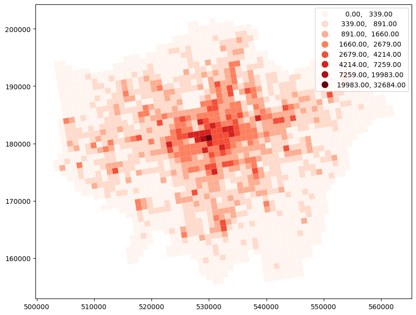
gdf_london_grid_poi_crime.plot(column= 'crime_counts', cmap='Reds', legend=True, k=8, scheme='FisherJenks', figsize=(10,8))
/Users/896604/miniconda3/envs/STBDA/lib/python3.10/site-packages/mapclassify/classifiers.py:1860: UserWarning: Numba not installed. Using slow pure python version.
  warnings.warn(
<Axes: >
Step 3 Data Splitting:
# Split the data into training and testing sets
from sklearn.model_selection import train_test_split
# Define the features (X) and target variable (y)
X = gdf_london_grid_poi_crime[['poi_counts', 'poi_types']]
y = gdf_london_grid_poi_crime['crime_counts']
# Split the data into training and testing sets (80% train, 20% test)
X_train, X_test, y_train, y_test = train_test_split(X, y, test_size=0.2, random_state=42)
# Check the shapes of the training and testing sets
print("X_train shape:", X_train.shape)
print("X_test shape:", X_test.shape)
print("y_train shape:", y_train.shape)
print("y_test shape:", y_test.shape)
X_train shape: (1386, 2)
X_test shape: (347, 2)
y_train shape: (1386,)
y_test shape: (347,)
Step 4 Feature Scaling:
# Feature scaling
from sklearn.preprocessing import StandardScaler
# Initialize the scaler
scaler = StandardScaler()
# Fit the scaler on the training data
scaler.fit(X_train)
# Transform the training and testing data
X_train_scaled = scaler.transform(X_train)
X_test_scaled = scaler.transform(X_test)
# Check the scaled data
print("X_train_scaled shape:", X_train_scaled.shape)
print("X_test_scaled shape:", X_test_scaled.shape)
# to transform the y train and y test data, reshape (-1,1) means to convert the 1D array to 2D array; this is required by the scaler
y_train_scaled = scaler.fit_transform(y_train.values.reshape(-1, 1))
y_test_scaled = scaler.transform(y_test.values.reshape(-1, 1))
# Check the scaled data
print("y_train_scaled shape:", y_train_scaled.shape)
print("y_test_scaled shape:", y_test_scaled.shape)
X_train_scaled shape: (1386, 2)
X_test_scaled shape: (347, 2)
y_train_scaled shape: (1386, 1)
y_test_scaled shape: (347, 1)
Step 5 Model Training and Hyperparameter Tuning (Cross-Validation):
#  train the SVM regression model and hyperparameter tuning using CV
from sklearn.svm import SVR
from sklearn.model_selection import GridSearchCV

# Define the SVM model
svm_model = SVR()
# Define the hyperparameters to tune
param_grid = {
    'kernel': ['linear', 'rbf', 'poly'],
    'C': [0.1, 1, 10, 100],
    'gamma': ['scale', 'auto', 0.1, 0.01],
    'epsilon': [0.1, 0.2, 0.3]
}
RandomizedSearchCV and GridSearchCV
# Perform grid search with cross-validation, here we use 5-fold CV and negative mean squared error as the scoring metric
grid_search = GridSearchCV(svm_model, param_grid, cv=5, scoring='neg_mean_squared_error', n_jobs=-1)
# there are 4 types of parameters set with 3, 4, 4, 3 selections in the param_grid, so the total number of combinations is 4*3*4*3 = 144;
# considering the 5-fold CV, the total number of models to be trained is 144*5 = 720
# ravel() is used to convert the 2D array to 1D array, this is required by the grid search
grid_search.fit(X_train_scaled, y_train_scaled.ravel())
# print the performance metrics
print("Best cross-validation score (MSE):", -grid_search.best_score_)
Best cross-validation score (MSE): 0.3469068801108338
gscv_results_df = pd.DataFrame(grid_search.cv_results_)
gscv_results_df
| mean_fit_time | std_fit_time | mean_score_time | std_score_time | param_C | param_epsilon | param_gamma | param_kernel | params | split0_test_score | split1_test_score | split2_test_score | split3_test_score | split4_test_score | mean_test_score | std_test_score | rank_test_score | |
|---|---|---|---|---|---|---|---|---|---|---|---|---|---|---|---|---|---|
| 0 | 0.014670 | 0.003606 | 0.001402 | 0.000076 | 0.1 | 0.1 | scale | linear | {'C': 0.1, 'epsilon': 0.1, 'gamma': 'scale', '... | -0.161602 | -0.309483 | -0.269594 | -0.213100 | -1.038503 | -0.398456 | 0.323925 | 39 |
| 1 | 0.015693 | 0.003923 | 0.004752 | 0.000310 | 0.1 | 0.1 | scale | rbf | {'C': 0.1, 'epsilon': 0.1, 'gamma': 'scale', '... | -0.178756 | -0.425421 | -0.337690 | -0.235625 | -1.408892 | -0.517277 | 0.453782 | 119 |
| 2 | 0.046964 | 0.009909 | 0.001963 | 0.000640 | 0.1 | 0.1 | scale | poly | {'C': 0.1, 'epsilon': 0.1, 'gamma': 'scale', '... | -0.235991 | -0.381201 | -0.431818 | -0.278688 | -0.515603 | -0.368660 | 0.101424 | 6 |
| 3 | 0.012760 | 0.002559 | 0.001370 | 0.000068 | 0.1 | 0.1 | auto | linear | {'C': 0.1, 'epsilon': 0.1, 'gamma': 'auto', 'k... | -0.161602 | -0.309483 | -0.269594 | -0.213100 | -1.038503 | -0.398456 | 0.323925 | 39 |
| 4 | 0.015724 | 0.002159 | 0.004598 | 0.000059 | 0.1 | 0.1 | auto | rbf | {'C': 0.1, 'epsilon': 0.1, 'gamma': 'auto', 'k... | -0.179099 | -0.424231 | -0.337557 | -0.236367 | -1.408735 | -0.517198 | 0.453636 | 118 |
| ... | ... | ... | ... | ... | ... | ... | ... | ... | ... | ... | ... | ... | ... | ... | ... | ... | ... |
| 139 | 0.024504 | 0.001720 | 0.002951 | 0.001099 | 100.0 | 0.3 | 0.1 | rbf | {'C': 100, 'epsilon': 0.3, 'gamma': 0.1, 'kern... | -0.189447 | -0.327770 | -0.273917 | -0.211199 | -1.403278 | -0.481122 | 0.463628 | 97 |
| 140 | 0.123786 | 0.031712 | 0.001063 | 0.000090 | 100.0 | 0.3 | 0.1 | poly | {'C': 100, 'epsilon': 0.3, 'gamma': 0.1, 'kern... | -0.228806 | -0.361929 | -0.396099 | -0.261518 | -1.036504 | -0.456971 | 0.296263 | 74 |
| 141 | 0.099407 | 0.017301 | 0.000878 | 0.000061 | 100.0 | 0.3 | 0.01 | linear | {'C': 100, 'epsilon': 0.3, 'gamma': 0.01, 'ker... | -0.169583 | -0.301983 | -0.259907 | -0.212265 | -1.041531 | -0.397054 | 0.325296 | 23 |
| 142 | 0.013884 | 0.003764 | 0.002413 | 0.000245 | 100.0 | 0.3 | 0.01 | rbf | {'C': 100, 'epsilon': 0.3, 'gamma': 0.01, 'ker... | -0.157879 | -0.318991 | -0.271800 | -0.206021 | -1.139578 | -0.418854 | 0.364540 | 64 |
| 143 | 0.015400 | 0.005429 | 0.001108 | 0.000058 | 100.0 | 0.3 | 0.01 | poly | {'C': 100, 'epsilon': 0.3, 'gamma': 0.01, 'ker... | -0.300499 | -0.815115 | -0.488829 | -0.297477 | -2.221372 | -0.824658 | 0.723373 | 137 |
144 rows × 17 columns
# get the best model from the grid search
best_model = grid_search.best_estimator_
# We can generate MSE manually and other performance metrics in the training set
from sklearn.metrics import mean_squared_error, r2_score, mean_absolute_error
# Make predictions on the training set
y_train_pred = best_model.predict(X_train_scaled)
# Calculate performance metrics
mse_train = mean_squared_error(y_train_scaled, y_train_pred)
mae_train = mean_absolute_error(y_train_scaled, y_train_pred)
r2_train = r2_score(y_train_scaled, y_train_pred)
print("Training set performance metrics:")
print("Mean Squared Error (MSE):", mse_train)
print("Mean Absolute Error (MAE):", mae_train)
print("R-squared (R2):", r2_train)
Training set performance metrics:
Mean Squared Error (MSE): 0.30264185557747325
Mean Absolute Error (MAE): 0.3689697950764123
R-squared (R2): 0.6973581444225267
# Get the best hyperparameters
best_params = grid_search.best_params_
print("Best hyperparameters:", best_params)
# Get the best model
best_model = grid_search.best_estimator_
Best hyperparameters: {'C': 10, 'epsilon': 0.3, 'gamma': 0.1, 'kernel': 'poly'}
Step 6 Model evaluation and testing:
# Make predictions on the test set
y_test_pred = best_model.predict(X_test_scaled)
# Calculate performance metrics
mse_test = mean_squared_error(y_test_scaled, y_test_pred)
mae_test = mean_absolute_error(y_test_scaled, y_test_pred)
r2_test = r2_score(y_test_scaled, y_test_pred)
print("Test set performance metrics:")
print("Mean Squared Error (MSE):", mse_test)
print("Mean Absolute Error (MAE):", mae_test)
print("R-squared (R2):", r2_test)
Test set performance metrics:
Mean Squared Error (MSE): 0.5879835533727016
Mean Absolute Error (MAE): 0.39449333359072636
R-squared (R2): 0.8348198471666948
8.2.2 Evaluating the trained SVR via random CV and Spatial CV#
Further discussion: is this trained SVR model robust in the context of spatial prediction?
We have previously discussed spatial CV and its importance. Here, the random CV may cause data leakage issues when splitting the original traning data into a new training set (80%) and new test/validation set (20%) from the original training data. We will analyze and compare the differences of trained SVR performance between random CV and spatial CV.
from sklearn.model_selection import KFold
from sklearn.metrics import mean_squared_error
import numpy as np
# random state is used to ensure the reproducibility of the random split, which means the same random seed will generate the same random numbers
kf = KFold(n_splits=5, shuffle=True, random_state=42)

mse_list = []
tr_idx_list = []
va_idx_list = []
for i, (train_idx, va_idx) in enumerate(kf.split(X_train_scaled)):
    X_tr, X_va = X_train_scaled[train_idx], X_train_scaled[va_idx]
    y_tr, y_va = y_train_scaled[train_idx], y_train_scaled[va_idx]
    # two ** means to unpack the dictionary as keyword arguments,
    model = svm_model.set_params(**{'C': 10, 'epsilon': 0.3, 'gamma': 0.1, 'kernel': 'poly'})
    model.fit(X_tr, y_tr.ravel())
    preds = model.predict(X_va)
    mse = mean_squared_error(y_va, preds)
    print(f"Fold {i+1}: MSE = {mse:.2f},",
          f"Training samples length = {len(train_idx.tolist())},",
          f"Validation samples length = {len(va_idx.tolist())}")
    mse_list.append(mse)
    print('Mean of mses:', f'{np.mean(mse_list):.2f}')
    tr_idx_list.append(train_idx.tolist())
    va_idx_list.append(va_idx.tolist())
Fold 1: MSE = 0.51, Training samples length = 1108, Validation samples length = 278
Mean of mses: 0.51
Fold 2: MSE = 0.34, Training samples length = 1109, Validation samples length = 277
Mean of mses: 0.42
Fold 3: MSE = 0.29, Training samples length = 1109, Validation samples length = 277
Mean of mses: 0.38
Fold 4: MSE = 0.41, Training samples length = 1109, Validation samples length = 277
Mean of mses: 0.39
Fold 5: MSE = 0.27, Training samples length = 1109, Validation samples length = 277
Mean of mses: 0.36
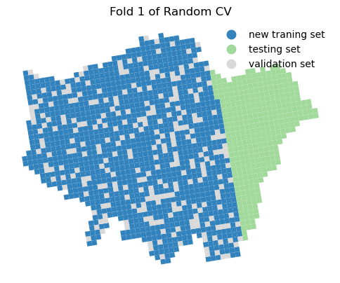
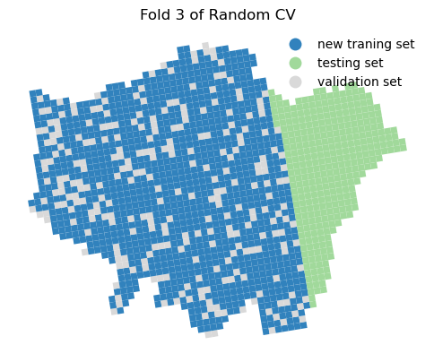
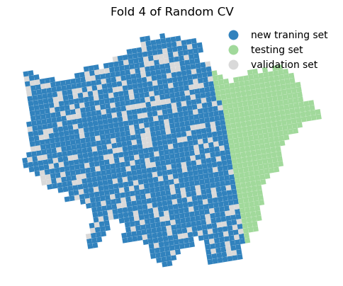
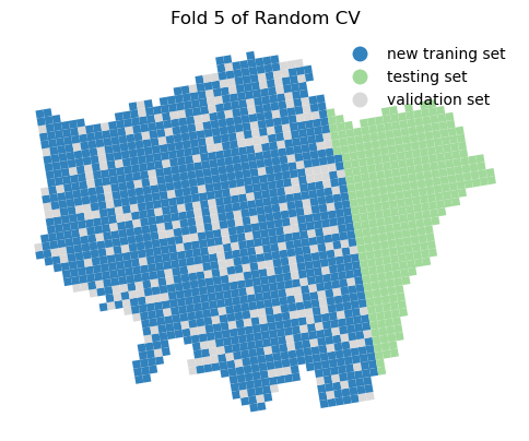
# we integrate the training and validation indices into the gdf for plotting
for i in range(0, 5):
    gdf_london_grid_poi_crime[f'index_gr'] = gdf_london_grid_poi_crime.index
    gdf_london_grid_poi_crime[f'Fold {i + 1}'] = gdf_london_grid_poi_crime.index_gr.apply(
        lambda x: 'new traning set' if x in tr_idx_list[i] else (
            'validation set' if x in va_idx_list[i] else 'testing set'))

    # we plot the train and test via the index on the grids
    fig, ax = plt.subplots(1, 1, figsize=(6, 6))
    gdf_london_grid_poi_crime.plot(ax=ax, column=f'Fold {i + 1}', cmap='tab20c', legend=True, figsize=(8, 6),
                                   legend_kwds={'frameon': False})
    plt.title(f'Fold {i + 1} of Random CV')
    ax.axis('off')
    plt.show()

# let us use a spatial CV through a k-means clustering to seprate the grids to 5 groups according to the coordinates
from sklearn.cluster import KMeans
# Define the number of clusters
n_clusters = 5
# Create a KMeans object
kmeans = KMeans(n_clusters=n_clusters, random_state=42)
# Fit the KMeans model according to the x and y coordinates of the grid centroids
gdf_london_grid_poi_crime['centroid_x'] = gdf_london_grid_poi_crime.geometry.centroid.x
gdf_london_grid_poi_crime['centroid_y'] = gdf_london_grid_poi_crime.geometry.centroid.y
# we don't use the testing set for clustering
gdf_london_grid_poi_crime_train = gdf_london_grid_poi_crime.loc[
    gdf_london_grid_poi_crime['Fold 1'] != 'testing set'].copy()
# Fit the KMeans model to the training data
kmeans.fit(gdf_london_grid_poi_crime_train[['centroid_x', 'centroid_y']])
# Assign cluster labels to the training data
gdf_london_grid_poi_crime_train.loc[:, 'cluster'] = kmeans.labels_
# we plot the clusters
fig, ax = plt.subplots(1, 1, figsize=(6, 6))
gdf_london_grid_poi_crime_train.plot(ax=ax, column='cluster')
<Axes: >

gdf_london_grid_poi_crime_train
| OBJECTID | grd_fixid | grd_floaid | grd_newid | pcd_count | tot_p | tot_m | tot_f | tot_hh | GlobalID | ... | crime_counts | index_gr | Fold 1 | Fold 2 | Fold 3 | Fold 4 | Fold 5 | centroid_x | centroid_y | cluster | |
|---|---|---|---|---|---|---|---|---|---|---|---|---|---|---|---|---|---|---|---|---|---|
| 0 | 214289 | 4.0.35930000.32030000 | 3593.3203.4 | 1kmN3203E3593 | 3 | 9 | 5 | 4 | 5 | 9f0c1e1f-e8fa-40ca-a969-d1aedbefa750 | ... | 5.0 | 0 | new traning set | new traning set | validation set | new traning set | new traning set | 503481.416280 | 175573.572278 | 2 |
| 1 | 214290 | 4.0.35930000.32040000 | 3593.3204.4 | 1kmN3204E3593 | 54 | 1957 | 1029 | 928 | 833 | e2530627-9630-4200-ae13-788341456d76 | ... | 13.0 | 1 | new traning set | new traning set | new traning set | new traning set | validation set | 503318.092908 | 176558.231134 | 2 |
| 2 | 214865 | 4.0.35940000.32020000 | 3594.3202.4 | 1kmN3202E3594 | 13 | 445 | 223 | 222 | 169 | bf801f98-5376-4c37-8bcb-d80ae9af1f0b | ... | 0.0 | 2 | new traning set | new traning set | validation set | new traning set | new traning set | 504632.628333 | 174752.571059 | 2 |
| 3 | 214866 | 4.0.35940000.32030000 | 3594.3203.4 | 1kmN3203E3594 | 3 | 34 | 18 | 16 | 11 | 472a8640-40e0-4c94-8eb5-37647847dc99 | ... | 1519.0 | 3 | new traning set | validation set | new traning set | new traning set | new traning set | 504469.320044 | 175737.238521 | 2 |
| 4 | 214867 | 4.0.35940000.32040000 | 3594.3204.4 | 1kmN3204E3594 | 1 | 15 | 9 | 6 | 8 | c21982c0-0d13-43df-8fa5-f77c28fba3d6 | ... | 0.0 | 4 | new traning set | new traning set | new traning set | validation set | new traning set | 504305.994245 | 176721.903963 | 2 |
| ... | ... | ... | ... | ... | ... | ... | ... | ... | ... | ... | ... | ... | ... | ... | ... | ... | ... | ... | ... | ... | ... |
| 1381 | 233221 | 4.0.36330000.32050000 | 3633.3205.4 | 1kmN3205E3633 | 149 | 17774 | 9897 | 7877 | 4810 | 81df1f73-eabc-432a-96cf-354e3b7e1e58 | ... | 3716.0 | 1381 | new traning set | new traning set | validation set | new traning set | new traning set | 542669.454612 | 184090.745646 | 1 |
| 1382 | 233222 | 4.0.36330000.32060000 | 3633.3206.4 | 1kmN3206E3633 | 138 | 17822 | 9494 | 8328 | 4784 | c5616e02-895d-4669-8768-8357a13dd7f2 | ... | 1345.0 | 1382 | new traning set | validation set | new traning set | new traning set | new traning set | 542506.025965 | 185075.698136 | 1 |
| 1383 | 233223 | 4.0.36330000.32070000 | 3633.3207.4 | 1kmN3207E3633 | 55 | 6018 | 3233 | 2785 | 1854 | 8f730656-d48d-4f99-928b-30cb304f3058 | ... | 861.0 | 1383 | new traning set | new traning set | new traning set | new traning set | validation set | 542342.579758 | 186060.646425 | 1 |
| 1384 | 233224 | 4.0.36330000.32080000 | 3633.3208.4 | 1kmN3208E3633 | 19 | 1544 | 734 | 810 | 529 | 40f56c08-6faf-46f0-b86f-43a4633d560e | ... | 152.0 | 1384 | new traning set | new traning set | new traning set | validation set | new traning set | 542179.116799 | 187045.595039 | 1 |
| 1385 | 233225 | 4.0.36330000.32090000 | 3633.3209.4 | 1kmN3209E3633 | 68 | 4602 | 2308 | 2294 | 1387 | 65b9480d-a4f7-4b82-9731-65080d9b5f31 | ... | 419.0 | 1385 | new traning set | new traning set | validation set | new traning set | new traning set | 542015.638307 | 188030.545768 | 1 |
1386 rows × 36 columns
Now we calculate the model performance in the training set using spatial CV, here we use the GroupKFold from sklearn.
# use groupcv in sklearn to select the data
from sklearn.model_selection import GroupKFold

# Define the number of splits
n_splits = 5
# Create a GroupKFold object
group_kfold = GroupKFold(n_splits=n_splits)
# Initialize an empty list to store the mean squared errors
g_mse_list = []
# Initialize an empty list to store the training and validation indices
g_tr_idx_list = []
g_va_idx_list = []
# Loop through the splits
for i, (g_train_idx, g_va_idx) in enumerate(
        group_kfold.split(X_train_scaled, y_train_scaled, groups=gdf_london_grid_poi_crime_train['cluster'])):
    X_tr, X_va = X_train_scaled[g_train_idx], X_train_scaled[g_va_idx]
    y_tr, y_va = y_train_scaled[g_train_idx], y_train_scaled[g_va_idx]
    model = svm_model.set_params(**{'C': 10, 'epsilon': 0.3, 'gamma': 0.1, 'kernel': 'poly'})
    model.fit(X_tr, y_tr.ravel())
    preds = model.predict(X_va)
    g_mse = mean_squared_error(y_va, preds)
    print(f"Fold {i + 1}: MSE = {g_mse:.2f}",
          f"Training samples length = {len(train_idx.tolist())},",
          f"Validation samples length = {len(va_idx.tolist())}")
    g_mse_list.append(g_mse)
    print('Mean of mses:', f'{np.mean(g_mse_list):.2f}')
    g_tr_idx_list.append(g_train_idx.tolist())
    g_va_idx_list.append(g_va_idx.tolist())
Fold 1: MSE = 0.31 Training samples length = 1109, Validation samples length = 277
Mean of mses: 0.31
Fold 2: MSE = 0.36 Training samples length = 1109, Validation samples length = 277
Mean of mses: 0.34
Fold 3: MSE = 0.36 Training samples length = 1109, Validation samples length = 277
Mean of mses: 0.35
Fold 4: MSE = 0.76 Training samples length = 1109, Validation samples length = 277
Mean of mses: 0.45
Fold 5: MSE = 0.24 Training samples length = 1109, Validation samples length = 277
Mean of mses: 0.41
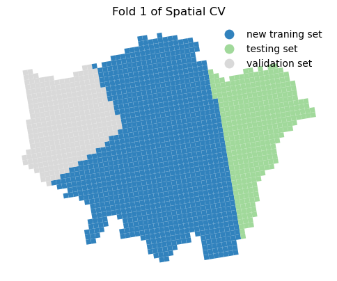
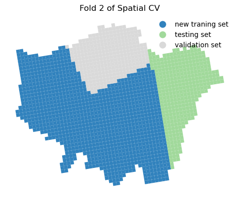
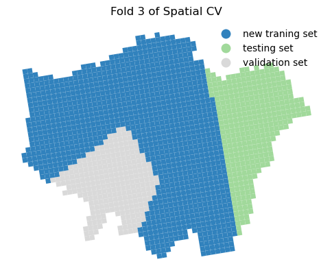
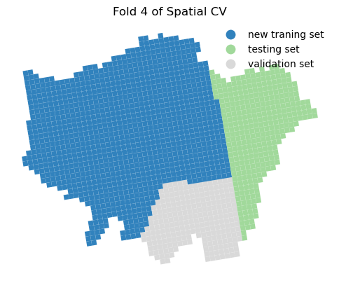
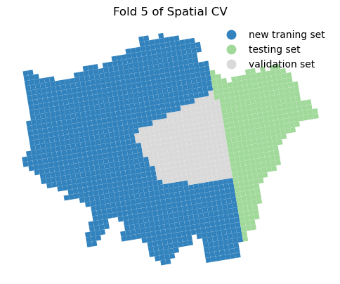
Mean of mses (0.41) is higher than the random CV (0.36), which means the model performance is worse via the spatial CV than the random CV.
# We integrate the training and validation indices into the gdf for plotting
for i in range(0, 5):
    gdf_london_grid_poi_crime[f'index_gr'] = gdf_london_grid_poi_crime.index
    gdf_london_grid_poi_crime[f'Group Fold {i + 1}'] = gdf_london_grid_poi_crime.index_gr.apply(
        lambda x: 'new traning set' if x in g_tr_idx_list[i] else (
            'validation set' if x in g_va_idx_list[i] else 'testing set'))
    # we plot the train and test via the index on the grids
    fig, ax = plt.subplots(1, 1, figsize=(6, 6))
    gdf_london_grid_poi_crime.plot(ax=ax, column=f'Group Fold {i + 1}', cmap='tab20c', legend=True, figsize=(8, 6),
                                   legend_kwds={'frameon': False})
    plt.title(f'Fold {i + 1} of Spatial CV')
    ax.axis('off')
    plt.show()
8.2.3 Retrain the SVR model and hyperparameter using GridSearch and Spatial CV#
Two important parameter settings in grid_search.fit() and GridSearchCV():
cv: this should be defined as the group_kfold from the
GroupKFoldgroups: this should be defined as the array/list groups_label from the training set
groups_label = gdf_london_grid_poi_crime_train['cluster'].values
Hyperparameter via GridSearch and Spatial CV
# Perform grid search with cross-validation, here we use 5-fold CV and negative mean squared error as the scoring metric
grid_search = GridSearchCV(svm_model, param_grid, cv=group_kfold, scoring='neg_mean_squared_error', n_jobs=-1)
# there are 4 types of parameters set with 3, 4, 4, 3 selections in the param_grid, so the total number of combinations is 4*3*4*3 = 144;
# considering the 5-fold CV, the total number of models to be trained is 144*5 = 720
# ravel() is used to convert the 2D array to 1D array, this is required by the grid search
grid_search.fit(X_train_scaled, y_train_scaled.ravel(), groups=groups_label)
# print the performance metrics
print("Best cross-validation score (MSE):", -grid_search.best_score_)
Best cross-validation score (MSE): 0.3880810150439128
Training set performance metrics
# get the best model from gridsearch and spatial cv
best_model_scv = grid_search.best_estimator_
# We can generate MSE manually and other performance metrics in the training set
from sklearn.metrics import mean_squared_error, r2_score, mean_absolute_error
# Make predictions on the training set
y_train_pred = best_model_scv.predict(X_train_scaled)
# Calculate performance metrics
mse_train = mean_squared_error(y_train_scaled, y_train_pred)
mae_train = mean_absolute_error(y_train_scaled, y_train_pred)
r2_train = r2_score(y_train_scaled, y_train_pred)
print("Training set performance metrics:")
print("Mean Squared Error (MSE):", mse_train)
print("Mean Absolute Error (MAE):", mae_train)
print("R-squared (R2):", r2_train)

# Get the best hyperparameters
best_params = grid_search.best_params_
print("Best hyperparameters:", best_params)
Training set performance metrics:
Mean Squared Error (MSE): 0.32209763512058076
Mean Absolute Error (MAE): 0.3537723982700458
R-squared (R2): 0.6779023648794191
Best hyperparameters: {'C': 10, 'epsilon': 0.1, 'gamma': 0.1, 'kernel': 'poly'}
Testing set performance metrics
# Make predictions on the test set
y_test_pred = best_model_scv.predict(X_test_scaled)
# Calculate performance metrics
mse_test = mean_squared_error(y_test_scaled, y_test_pred)
mae_test = mean_absolute_error(y_test_scaled, y_test_pred)
r2_test = r2_score(y_test_scaled, y_test_pred)
print("Test set performance metrics:")
print("Mean Squared Error (MSE):", mse_test)
print("Mean Absolute Error (MAE):", mae_test)
print("R-squared (R2):", r2_test)
Test set performance metrics:
Mean Squared Error (MSE): 0.6321250775477194
Mean Absolute Error (MAE): 0.3746731427775627
R-squared (R2): 0.8224193239416807
We observe that the model’s performance decreases when using spatial cross-validation and grid search compared to the random cross-validation approach. Additionally, the optimal hyperparameters have changed. This suggests that, in the context of spatial prediction, the current model is more robust than the one we previously trained, even though its overall performance appears to be lower.
Future work could include incorporating additional spatial features we previously calculated, such as spatial lags of all variables and LISA. Additionally, including more feature data may help improve the model’s performance.
8.3 Random Forests (RF) in the spatial and temporal prediction task#
Random Forests (RF) is an ensemble learning method that combines multiple decision trees to improve predictive accuracy and control overfitting. It is widely used for both classification and regression tasks. Key parameters in RF include:
n_estimators: The number of trees in the forest. More trees can lead to better performance but also increase computation time.
max_depth: The maximum depth of each tree. Limiting depth can help prevent overfitting.
min_samples_split: The minimum number of samples required to split an internal node. Higher values can lead to more conservative trees.
min_samples_leaf: The minimum number of samples required to be at a leaf node. Higher values can help smooth the model.
max_features: The number of features to consider when looking for the best split. It can be set to a fraction of the total number of features or a specific number.
Random Forests can be also used in feature engineering, such as feature importance ranking (Gini index), which helps identify the most relevant features for the prediction task.
We will use the same data as in the SVM section, but we will use the Random Forests model in a spatial and temporal prediction task: we use the first 11 months of crime data (2024-01 to 2024-11) to predict the crime level in December 2024. The features are the same as in the SVM section, i.e., the POI data.
# re-load the gdf_london_grid_poi_crime data
gdf_london_grid_poi_crime = gpd.read_file('data/london_grid_poi_crime.geojson')
gdf_london_grid_poi_crime
| OBJECTID | grd_fixid | grd_floaid | grd_newid | pcd_count | tot_p | tot_m | tot_f | tot_hh | GlobalID | ... | 2024-05 | 2024-06 | 2024-07 | 2024-08 | 2024-09 | 2024-10 | 2024-11 | 2024-12 | crime_counts | geometry | |
|---|---|---|---|---|---|---|---|---|---|---|---|---|---|---|---|---|---|---|---|---|---|
| 0 | 214289 | 4.0.35930000.32030000 | 3593.3203.4 | 1kmN3203E3593 | 3 | 9 | 5 | 4 | 5 | 9f0c1e1f-e8fa-40ca-a969-d1aedbefa750 | ... | 3.0 | 0.0 | 0.0 | 0.0 | 0.0 | 0.0 | 0.0 | 1.0 | 5.0 | POLYGON ((-0.50339 51.46588, -0.51765 51.46459... |
| 1 | 214290 | 4.0.35930000.32040000 | 3593.3204.4 | 1kmN3204E3593 | 54 | 1957 | 1029 | 928 | 833 | e2530627-9630-4200-ae13-788341456d76 | ... | 1.0 | 0.0 | 0.0 | 4.0 | 2.0 | 0.0 | 1.0 | 1.0 | 13.0 | POLYGON ((-0.50545 51.47476, -0.51972 51.47347... |
| 2 | 214865 | 4.0.35940000.32020000 | 3594.3202.4 | 1kmN3202E3594 | 13 | 445 | 223 | 222 | 169 | bf801f98-5376-4c37-8bcb-d80ae9af1f0b | ... | 0.0 | 0.0 | 0.0 | 0.0 | 0.0 | 0.0 | 0.0 | 0.0 | 0.0 | POLYGON ((-0.48707 51.45829, -0.50133 51.457, ... |
| 3 | 214866 | 4.0.35940000.32030000 | 3594.3203.4 | 1kmN3203E3594 | 3 | 34 | 18 | 16 | 11 | 472a8640-40e0-4c94-8eb5-37647847dc99 | ... | 126.0 | 105.0 | 124.0 | 134.0 | 127.0 | 137.0 | 141.0 | 124.0 | 1519.0 | POLYGON ((-0.48913 51.46717, -0.50339 51.46588... |
| 4 | 214867 | 4.0.35940000.32040000 | 3594.3204.4 | 1kmN3204E3594 | 1 | 15 | 9 | 6 | 8 | c21982c0-0d13-43df-8fa5-f77c28fba3d6 | ... | 0.0 | 0.0 | 0.0 | 0.0 | 0.0 | 0.0 | 0.0 | 0.0 | 0.0 | POLYGON ((-0.49118 51.47605, -0.50545 51.47476... |
| ... | ... | ... | ... | ... | ... | ... | ... | ... | ... | ... | ... | ... | ... | ... | ... | ... | ... | ... | ... | ... | ... |
| 1728 | 240548 | 4.0.36510000.32040000 | 3651.3204.4 | 1kmN3204E3651 | 0 | 0 | 0 | 0 | 0 | c1be8f1c-6c91-4dca-aad2-ce9f51538b0e | ... | 0.0 | 0.0 | 0.0 | 0.0 | 0.0 | 0.0 | 0.0 | 0.0 | 0.0 | POLYGON ((0.32328 51.54665, 0.30897 51.54546, ... |
| 1729 | 240549 | 4.0.36510000.32050000 | 3651.3205.4 | 1kmN3205E3651 | 2 | 73 | 41 | 32 | 25 | 65336bd5-772b-4398-a0de-4ccb1b438479 | ... | 0.0 | 0.0 | 0.0 | 0.0 | 0.0 | 0.0 | 0.0 | 0.0 | 0.0 | POLYGON ((0.32137 51.55555, 0.30706 51.55436, ... |
| 1730 | 240550 | 4.0.36510000.32060000 | 3651.3206.4 | 1kmN3206E3651 | 2 | 36 | 16 | 20 | 13 | befe6e14-0fef-4c44-8440-c3e80c139c63 | ... | 0.0 | 0.0 | 0.0 | 0.0 | 0.0 | 0.0 | 0.0 | 0.0 | 0.0 | POLYGON ((0.31947 51.56445, 0.30515 51.56326, ... |
| 1731 | 240929 | 4.0.36520000.32030000 | 3652.3203.4 | 1kmN3203E3652 | 2 | 26 | 15 | 11 | 12 | 96832cf0-62a9-49a4-b442-ac283b90db87 | ... | 0.0 | 0.0 | 1.0 | 0.0 | 0.0 | 2.0 | 0.0 | 0.0 | 3.0 | POLYGON ((0.33949 51.53894, 0.32518 51.53776, ... |
| 1732 | 240930 | 4.0.36520000.32040000 | 3652.3204.4 | 1kmN3204E3652 | 0 | 0 | 0 | 0 | 0 | f0c429cf-e001-432e-a41b-259a3c9e6582 | ... | 0.0 | 0.0 | 0.0 | 0.0 | 0.0 | 0.0 | 0.0 | 0.0 | 0.0 | POLYGON ((0.33759 51.54784, 0.32328 51.54665, ... |
1733 rows × 27 columns
# we need to reshape the df to have the columns: spatial index (grid), temporal index (month), X (poi_counts and poi_types) and y (crime_counts) as we need to predict the crime level in December 2024
df_X_y = gdf_london_grid_poi_crime.melt(id_vars=['grd_newid'],
                                          value_vars=[f'2024-{i:02d}' for i in range(1, 13)],
                                          var_name='Month', value_name='c_counts')
df_X_y.sort_values(by=['grd_newid', 'Month'], inplace=True)
df_X_y
| grd_newid | Month | c_counts | |
|---|---|---|---|
| 1048 | 1kmN3178E3626 | 2024-01 | 0.0 |
| 2781 | 1kmN3178E3626 | 2024-02 | 0.0 |
| 4514 | 1kmN3178E3626 | 2024-03 | 0.0 |
| 6247 | 1kmN3178E3626 | 2024-04 | 0.0 |
| 7980 | 1kmN3178E3626 | 2024-05 | 0.0 |
| ... | ... | ... | ... |
| 13137 | 1kmN3224E3624 | 2024-08 | 0.0 |
| 14870 | 1kmN3224E3624 | 2024-09 | 0.0 |
| 16603 | 1kmN3224E3624 | 2024-10 | 0.0 |
| 18336 | 1kmN3224E3624 | 2024-11 | 0.0 |
| 20069 | 1kmN3224E3624 | 2024-12 | 0.0 |
20796 rows × 3 columns
# make sure we have the all spatial and temporal unit of analysis
df_X_y.grd_newid.nunique() * df_X_y.Month.nunique()
20796
# attach the poi_counts and poi_types to the df_X_y
df_X_y = pd.merge(df_X_y, gdf_london_grid_poi_crime[['grd_newid', 'poi_counts', 'poi_types']],  on='grd_newid', how='left')
df_X_y
| grd_newid | Month | c_counts | poi_counts | poi_types | |
|---|---|---|---|---|---|
| 0 | 1kmN3178E3626 | 2024-01 | 0.0 | 0.0 | 0.0 |
| 1 | 1kmN3178E3626 | 2024-02 | 0.0 | 0.0 | 0.0 |
| 2 | 1kmN3178E3626 | 2024-03 | 0.0 | 0.0 | 0.0 |
| 3 | 1kmN3178E3626 | 2024-04 | 0.0 | 0.0 | 0.0 |
| 4 | 1kmN3178E3626 | 2024-05 | 0.0 | 0.0 | 0.0 |
| ... | ... | ... | ... | ... | ... |
| 20791 | 1kmN3224E3624 | 2024-08 | 0.0 | 0.0 | 0.0 |
| 20792 | 1kmN3224E3624 | 2024-09 | 0.0 | 0.0 | 0.0 |
| 20793 | 1kmN3224E3624 | 2024-10 | 0.0 | 0.0 | 0.0 |
| 20794 | 1kmN3224E3624 | 2024-11 | 0.0 | 0.0 | 0.0 |
| 20795 | 1kmN3224E3624 | 2024-12 | 0.0 | 0.0 | 0.0 |
20796 rows × 5 columns
# Selceting the training and testing data
# we use the first 11 months as the training data and the last month (December) as the testing data
df_X_y_train = df_X_y[df_X_y['Month'] != '2024-12']
df_X_y_test = df_X_y[df_X_y['Month'] == '2024-12']
X_train = df_X_y_train[['poi_counts', 'poi_types']]
y_train = df_X_y_train['c_counts']
X_test = df_X_y_test[['poi_counts', 'poi_types']]
y_test = df_X_y_test['c_counts']
# hyperparameter tuning using GridSearchCV in Random Forests
from sklearn.ensemble import RandomForestRegressor
from sklearn.model_selection import GridSearchCV
# Define the Random Forest model
rf_model = RandomForestRegressor(random_state=42)
# Define the hyperparameters to tune
param_grid_rf = {
    'n_estimators': [50, 100],
    'max_depth': [3, 5, 7, 10],
    'min_samples_split': [2, 5, 7],
    'min_samples_leaf': [1, 2, 6]}
# Perform grid search with cross-validation, here we use 5-fold CV and negative mean squared error as the scoring metric
grid_search_rf = GridSearchCV(rf_model, param_grid_rf, cv=5, scoring='neg_mean_squared_error', n_jobs=-1)
# Fit the model on the training data
grid_search_rf.fit(X_train, y_train)
# Print the best hyperparameters and the best score
print("Best hyperparameters:", grid_search_rf.best_params_)
print("Best cross-validation score (MSE):", -grid_search_rf.best_score_)
Best hyperparameters: {'max_depth': 5, 'min_samples_leaf': 1, 'min_samples_split': 7, 'n_estimators': 100}
Best cross-validation score (MSE): 6265.360893316517
# Get the best model from the grid search
best_rf_model = grid_search_rf.best_estimator_
# output the importance of the features
importances = best_rf_model.feature_importances_
feature_names = X_train.columns
# Create a DataFrame to hold feature names and their importance scores
feature_importance_df = pd.DataFrame({'Feature': feature_names, 'Importance': importances})
# Sort the DataFrame by importance scores in descending order
feature_importance_df = feature_importance_df.sort_values(by='Importance', ascending=False)
feature_importance_df
| Feature | Importance | |
|---|---|---|
| 0 | poi_counts | 0.574831 |
| 1 | poi_types | 0.425169 |
# Training set performance metrics
from sklearn.metrics import mean_squared_error, r2_score, mean_absolute_error
# Make predictions on the training set
y_train_pred_rf = best_rf_model.predict(X_train)
# Calculate performance metrics
mse_train_rf = mean_squared_error(y_train, y_train_pred_rf)
mae_train_rf = mean_absolute_error(y_train, y_train_pred_rf)
r2_train_rf = r2_score(y_train, y_train_pred_rf)
print("Training set performance metrics:")
print("Mean Squared Error (MSE):", mse_train_rf)
print("Mean Absolute Error (MAE):", mae_train_rf)
print("R-squared (R2):", r2_train_rf)
Training set performance metrics:
Mean Squared Error (MSE): 1576.2537522196371
Mean Absolute Error (MAE): 24.499505744829683
R-squared (R2): 0.8532881379884858
# Testing set performance metrics
# Make predictions on the test set
y_test_pred_rf = best_rf_model.predict(df_X_y_test[['poi_counts', 'poi_types']])
# Calculate performance metrics
mse_test_rf = mean_squared_error(y_test, y_test_pred_rf)
mae_test_rf = mean_absolute_error(y_test, y_test_pred_rf)
r2_test_rf = r2_score(y_test, y_test_pred_rf)
print("Test set performance metrics:")
print("Mean Squared Error (MSE):", mse_test_rf)
print("Mean Absolute Error (MAE):", mae_test_rf)
print("R-squared (R2):", r2_test_rf)
Test set performance metrics:
Mean Squared Error (MSE): 2058.6680182257987
Mean Absolute Error (MAE): 23.931832242381546
R-squared (R2): 0.8598031898525247
Quiz#
Q1: Use the same data in the Random Forests section, but use the SVM model to predict the crime level in December 2024. Use the same hyperparameter tuning method (GridsearchCV) as in the Random Forests section. Compare the performance of the SVM model with the Random Forests model.
Q2: Use the same data in the Random Forests section, but use the GWR model to predict the crime level in December 2024. Compare the performance of the GWR model with the Random Forests model.
Q1 solution:
from sklearn.svm import SVR
# Define the SVM model
svm_model = SVR()
# Define the hyperparameters to tune
param_grid_svm = {
    'kernel': ['linear', 'rbf'],
    'C': [0.1, 1, 10],
    'gamma': [0.1, 0.01],
    'epsilon': [0.1,0.3]
}
# Perform grid search with cross-validation, here we use 5-fold CV and negative mean squared error as the scoring metric
grid_search_svm = GridSearchCV(svm_model, param_grid_svm, cv=5, scoring='neg_mean_squared_error', n_jobs=-1)
# Fit the model on the training data
grid_search_svm.fit(X_train, y_train)
# Print the best hyperparameters and the best score
print("Best hyperparameters:", grid_search_svm.best_params_)
print("Best cross-validation score (MSE):", -grid_search_svm.best_score_)
# Get the best model from the grid search
best_svm_model = grid_search_svm.best_estimator_
/Users/896604/miniconda3/envs/STBDA/lib/python3.10/site-packages/joblib/externals/loky/process_executor.py:752: UserWarning: A worker stopped while some jobs were given to the executor. This can be caused by a too short worker timeout or by a memory leak.
  warnings.warn(
Best hyperparameters: {'C': 0.1, 'epsilon': 0.1, 'gamma': 0.1, 'kernel': 'linear'}
Best cross-validation score (MSE): 5763.656583753928
# output the training set performance metrics
# Make predictions on the training set
y_train_pred_svm = best_svm_model.predict(X_train)
# Calculate performance metrics
mse_train_svm = mean_squared_error(y_train, y_train_pred_svm)
mae_train_svm = mean_absolute_error(y_train, y_train_pred_svm)
r2_train_svm = r2_score(y_train, y_train_pred_svm)
print("Training set performance metrics:")
print("Mean Squared Error (MSE):", mse_train_svm)
print("Mean Absolute Error (MAE):", mae_train_svm)
print("R-squared (R2):", r2_train_svm)
Training set performance metrics:
Mean Squared Error (MSE): 5172.553455303947
Mean Absolute Error (MAE): 27.01774179526304
R-squared (R2): 0.5185578795843584
# Testing set performance metrics
# Make predictions on the test set
y_test_pred_svm = best_svm_model.predict(X_test)
# Calculate performance metrics
mse_test_svm = mean_squared_error(y_test, y_test_pred_svm)
mae_test_svm = mean_absolute_error(y_test, y_test_pred_svm)
r2_test_svm = r2_score(y_test, y_test_pred_svm)
print("Test set performance metrics:")
print("Mean Squared Error (MSE):", mse_test_svm)
print("Mean Absolute Error (MAE):", mae_test_svm)
print("R-squared (R2):", r2_test_svm)
Test set performance metrics:
Mean Squared Error (MSE): 8500.947557530795
Mean Absolute Error (MAE): 26.248980252989444
R-squared (R2): 0.4210792025496609
Q2 solution:
df_X_y_train
| grd_newid | Month | c_counts | poi_counts | poi_types | |
|---|---|---|---|---|---|
| 0 | 1kmN3178E3626 | 2024-01 | 0.0 | 0.0 | 0.0 |
| 1 | 1kmN3178E3626 | 2024-02 | 0.0 | 0.0 | 0.0 |
| 2 | 1kmN3178E3626 | 2024-03 | 0.0 | 0.0 | 0.0 |
| 3 | 1kmN3178E3626 | 2024-04 | 0.0 | 0.0 | 0.0 |
| 4 | 1kmN3178E3626 | 2024-05 | 0.0 | 0.0 | 0.0 |
| ... | ... | ... | ... | ... | ... |
| 20790 | 1kmN3224E3624 | 2024-07 | 0.0 | 0.0 | 0.0 |
| 20791 | 1kmN3224E3624 | 2024-08 | 0.0 | 0.0 | 0.0 |
| 20792 | 1kmN3224E3624 | 2024-09 | 0.0 | 0.0 | 0.0 |
| 20793 | 1kmN3224E3624 | 2024-10 | 0.0 | 0.0 | 0.0 |
| 20794 | 1kmN3224E3624 | 2024-11 | 0.0 | 0.0 | 0.0 |
19063 rows × 5 columns
# we need to prepare the data for  GWR, which requires the coordinates and the features and target variables
df_coors = gdf_london_grid_poi_crime[['grd_newid', 'geometry']]
# transfer crs to uk grid system
df_coors = df_coors.to_crs(epsg=27700)
df_coors['east'] = df_coors.geometry.centroid.x
df_coors['north'] = df_coors.geometry.centroid.y
df_coors_s = df_coors[['grd_newid', 'east', 'north']]
# merge the coordinates with the training data
df_X_y_train = df_X_y_train.merge(df_coors_s, on='grd_newid', how='left')
df_X_y_train
| grd_newid | Month | c_counts | poi_counts | poi_types | east | north | |
|---|---|---|---|---|---|---|---|
| 0 | 1kmN3178E3626 | 2024-01 | 0.0 | 0.0 | 0.0 | 540160.898592 | 156351.273341 |
| 1 | 1kmN3178E3626 | 2024-02 | 0.0 | 0.0 | 0.0 | 540160.898592 | 156351.273341 |
| 2 | 1kmN3178E3626 | 2024-03 | 0.0 | 0.0 | 0.0 | 540160.898592 | 156351.273341 |
| 3 | 1kmN3178E3626 | 2024-04 | 0.0 | 0.0 | 0.0 | 540160.898592 | 156351.273341 |
| 4 | 1kmN3178E3626 | 2024-05 | 0.0 | 0.0 | 0.0 | 540160.898592 | 156351.273341 |
| ... | ... | ... | ... | ... | ... | ... | ... |
| 19058 | 1kmN3224E3624 | 2024-07 | 0.0 | 0.0 | 0.0 | 530671.170943 | 201329.693106 |
| 19059 | 1kmN3224E3624 | 2024-08 | 0.0 | 0.0 | 0.0 | 530671.170943 | 201329.693106 |
| 19060 | 1kmN3224E3624 | 2024-09 | 0.0 | 0.0 | 0.0 | 530671.170943 | 201329.693106 |
| 19061 | 1kmN3224E3624 | 2024-10 | 0.0 | 0.0 | 0.0 | 530671.170943 | 201329.693106 |
| 19062 | 1kmN3224E3624 | 2024-11 | 0.0 | 0.0 | 0.0 | 530671.170943 | 201329.693106 |
19063 rows × 7 columns
from mgwr.gwr import GWR
from mgwr.sel_bw import Sel_BW

# Prepare data
coords = df_X_y_train[['east', 'north']].values               # shape (n_samples, 2)
X = df_X_y_train[['poi_counts', 'poi_types']].values          # shape (n_samples, n_features)
y = df_X_y_train[['c_counts']].values                         # shape (n_samples, 1)

# Bandwidth selection
sel_bw = Sel_BW(coords, y, X, fixed=False,  kernel='gaussian')
bw = sel_bw.search(bw_min=2, bw_max=100)
print(f"Selected bandwidth: {bw}")
# GWR model fitting
mgwr_model = GWR(coords, y, X, bw=bw, fixed=False,  kernel='gaussian')
results = mgwr_model.fit()  # assign to a variable!
Selected bandwidth: 25.0
import numpy as np
np.float = float # Monkey patch, as gwr.summary() relies on numpy version < 1.24
results.summary()
===========================================================================
Model type                                                         Gaussian
Number of observations:                                               19063
Number of covariates:                                                     3

Global Regression Results
---------------------------------------------------------------------------
Residual sum of squares:                                       77741310.342
Log-likelihood:                                                 -106288.329
AIC:                                                             212582.657
AICc:                                                            212584.659
BIC:                                                           77553464.425
R2:                                                                   0.620
Adj. R2:                                                              0.620

Variable                              Est.         SE  t(Est/SE)    p-value
------------------------------- ---------- ---------- ---------- ----------
X0                                   9.506      0.691     13.764      0.000
X1                                   0.890      0.009     99.121      0.000
X2                                  -0.225      0.062     -3.624      0.000

Geographically Weighted Regression (GWR) Results
---------------------------------------------------------------------------
Spatial kernel:                                           Adaptive gaussian
Bandwidth used:                                                      25.000

Diagnostic information
---------------------------------------------------------------------------
Residual sum of squares:                                       18810354.478
Effective number of parameters (trace(S)):                          598.280
Degree of freedom (n - trace(S)):                                 18464.720
Sigma estimate:                                                      31.917
Log-likelihood:                                                  -92763.327
AIC:                                                             186725.214
AICc:                                                            186764.183
BIC:                                                             191432.859
R2:                                                                   0.908
Adjusted R2:                                                          0.905
Adj. alpha (95%):                                                     0.000
Adj. critical t value (95%):                                          3.662

Summary Statistics For GWR Parameter Estimates
---------------------------------------------------------------------------
Variable                   Mean        STD        Min     Median        Max
-------------------- ---------- ---------- ---------- ---------- ----------
X0                        0.591     46.791   -976.165      3.646    259.681
X1                        0.200      0.832     -3.308      0.076      6.296
X2                        2.307      2.838    -14.226      2.116     11.568
===========================================================================
# predicting the December 2024 crime level
# In-sample prediction
y_train_predictions = mgwr_model.predict(coords, X)
# Calculate performance metrics for the training set
mse_train_mgwr = mean_squared_error(y, y_train_predictions.predictions)
mae_train_mgwr = mean_absolute_error(y, y_train_predictions.predictions)
r2_train_mgwr = r2_score(y, y_train_predictions.predictions)
print("Training set performance metrics:")
print("Mean Squared Error (MSE):", mse_train_mgwr)
print("Mean Absolute Error (MAE):", mae_train_mgwr)
print("R-squared (R2):", r2_train_mgwr)
Training set performance metrics:
Mean Squared Error (MSE): 986.74681202883
Mean Absolute Error (MAE): 15.172640017308824
R-squared (R2): 0.9081572608960851
df_X_y_test = df_X_y_test.merge(df_coors_s, on='grd_newid', how='left')
df_X_y_test
| grd_newid | Month | c_counts | poi_counts | poi_types | east | north | |
|---|---|---|---|---|---|---|---|
| 0 | 1kmN3178E3626 | 2024-12 | 0.0 | 0.0 | 0.0 | 540160.898592 | 156351.273341 |
| 1 | 1kmN3178E3627 | 2024-12 | 0.0 | 13.0 | 7.0 | 541148.801501 | 156514.772306 |
| 2 | 1kmN3178E3628 | 2024-12 | 0.0 | 1.0 | 1.0 | 542136.703610 | 156678.270809 |
| 3 | 1kmN3178E3629 | 2024-12 | 0.0 | 1.0 | 1.0 | 543124.604471 | 156841.769399 |
| 4 | 1kmN3178E3630 | 2024-12 | 0.0 | 1.0 | 1.0 | 544112.504850 | 157005.269369 |
| ... | ... | ... | ... | ... | ... | ... | ... |
| 1728 | 1kmN3223E3626 | 2024-12 | 0.0 | 0.0 | 0.0 | 532810.468008 | 200672.557618 |
| 1729 | 1kmN3223E3627 | 2024-12 | 0.0 | 0.0 | 0.0 | 533798.279960 | 200836.397365 |
| 1730 | 1kmN3224E3620 | 2024-12 | 0.0 | 5.0 | 4.0 | 526719.906430 | 200674.265154 |
| 1731 | 1kmN3224E3621 | 2024-12 | 0.0 | 1.0 | 1.0 | 527707.725648 | 200838.116449 |
| 1732 | 1kmN3224E3624 | 2024-12 | 0.0 | 0.0 | 0.0 | 530671.170943 | 201329.693106 |
1733 rows × 7 columns
coors_test = df_X_y_test[['east', 'north']].values
X_test = df_X_y_test[['poi_counts', 'poi_types']].values
y_test = df_X_y_test[['c_counts']].values
mgwr_model.bw
25.0
# Testing set performance metrics
gwr_test_model = GWR(coors_test, y_test, X_test, bw=25, fixed=False, kernel='gaussian')
results_test = gwr_test_model.fit()
import numpy as np
np.float = float # Monkey patch, as gwr.summary() relies on numpy version < 1.24
results_test.summary()
===========================================================================
Model type                                                         Gaussian
Number of observations:                                                1733
Number of covariates:                                                     3

Global Regression Results
---------------------------------------------------------------------------
Residual sum of squares:                                       10908510.231
Log-likelihood:                                                  -10038.681
AIC:                                                              20083.362
AICc:                                                             20085.385
BIC:                                                           10895608.567
R2:                                                                   0.571
Adj. R2:                                                              0.571

Variable                              Est.         SE  t(Est/SE)    p-value
------------------------------- ---------- ---------- ---------- ----------
X0                                  13.559      2.848      4.761      0.000
X1                                   1.186      0.037     32.022      0.000
X2                                  -1.891      0.256     -7.376      0.000

Geographically Weighted Regression (GWR) Results
---------------------------------------------------------------------------
Spatial kernel:                                           Adaptive gaussian
Bandwidth used:                                                      25.000

Diagnostic information
---------------------------------------------------------------------------
Residual sum of squares:                                        6830750.006
Effective number of parameters (trace(S)):                           85.372
Degree of freedom (n - trace(S)):                                  1647.628
Sigma estimate:                                                      64.388
Log-likelihood:                                                   -9633.065
AIC:                                                              19438.874
AICc:                                                             19448.046
BIC:                                                              19910.261
R2:                                                                   0.732
Adjusted R2:                                                          0.718
Adj. alpha (95%):                                                     0.002
Adj. critical t value (95%):                                          3.133

Summary Statistics For GWR Parameter Estimates
---------------------------------------------------------------------------
Variable                   Mean        STD        Min     Median        Max
-------------------- ---------- ---------- ---------- ---------- ----------
X0                       10.592     31.057    -55.690      4.272    246.785
X1                        0.383      0.511     -0.474      0.253      2.418
X2                        1.341      3.122    -14.972      1.886      5.325
===========================================================================
# In testing set prediction
y_test_predictions = gwr_test_model.predict(coors_test, X_test)
# Calculate performance metrics for the testing set
mse_test_mgwr = mean_squared_error(y_test, y_test_predictions.predictions)
mae_test_mgwr = mean_absolute_error(y_test, y_test_predictions.predictions)
r2_test_mgwr = r2_score(y_test, y_test_predictions.predictions)
print("Testing set performance metrics:")
print("Mean Squared Error (MSE):", mse_test_mgwr)
print("Mean Absolute Error (MAE):", mae_test_mgwr)
print("R-squared (R2):", r2_test_mgwr)
Testing set performance metrics:
Mean Squared Error (MSE): 3941.575306423653
Mean Absolute Error (MAE): 26.264055429467643
R-squared (R2): 0.7315758150297141