Week5 Lab Tutorial Timeline
Time |
Activity |
|---|---|
16:00–16:05 |
Introduction — Overview of the main tasks for the lab tutorials |
16:05–16:45 |
Tutorial: geospatial modelling 1 — Follow Section 5.1-5.3 of the Jupyter Notebook to practice the spatial lag, SLM, SEM |
16:45–17:30 |
Tutorial: geospatial modelling 2 — Follow Section 5.4-5.6 of the Jupyter Notebook to practice the SDM, GWR and mGWR |
17:30–17:55 |
Quiz — Complete quiz tasks |
17:55–18:00 |
Wrap-up — Recap key points and address final questions |
For this module’s lab tutorials, you can download all the required data using the provided link (click).
Please make sure that both the Jupyter Notebook file and the data and img folder are placed in the same directory (specifically within the STBDA_lab folder) to ensure the code runs correctly.
Week 5 Key Takeaways:
Understand the spatial lags and compute using libpysal;
Understand and perform the SLM model;
Understand and perform the SEM model;
Understand and perform the SDM model;
Understand and perform the GWR and mGWR model.
5 Geospatial statistical modelling#
Spatial regression is a type of statistical modeling that accounts for spatial dependence (when nearby locations influence each other) and spatial heterogeneity (when the distribution of a single variable and relationships between variables vary across space) in the data. In other words, it’s used when geolocation matters and traditional regression methods (like OLS) might give misleading results due to spatial dependence or spatial heterogeneity.
# Import the required libraries
import numpy as np
import esda
import geopandas as gpd
import libpysal.weights as weights
import matplotlib.pyplot as plt
import pandas as pd
import warnings
warnings.filterwarnings("ignore")
5.1 Spatial lag#
Spatial lag refers to a weighted measurement of neighboring values (based on a spatial weights matrix). It captures how a variable at one location is influenced by its neighbors. In other words, spatial lag helps capture spatial dependence — where values in one area depend on values in neighboring areas/units.
Spatial lag as a new variable is popularly used as a predictor in spatial regression models.
The spatial lag of a variable \(y\) is calculated as:
Where:
\(y\) is the vector of the variable you’re analyzing (e.g., income, house price)
\(W\) is the spatial weights matrix, which defines how locations relate to each other (e.g., neighbors)
\(Wy\) is the spatial lag, a new vector where each element is the weighted sum of neighboring \(y\) values
Each element \((Wy)_i\) is computed as:
Where:
\(w_{ij}\) is the spatial weight between location \(i\) and neighbor \(j\)
\(y_j\) is the value of the variable \(y\) at location \(j\)
We use the defination above to calculate the spatial lag manually or use libpysal library to compute the spatial lag for the crime incidents in London LSOAs used before.
gdf_crime_agg_may = gpd.read_file('data/gdf_crime_agg_may.geojson')
gdf_crime_agg_may
| LSOA21CD | Month | Count | Z_score | p_sim | geometry | |
|---|---|---|---|---|---|---|
| 0 | E01000001 | 2024-05 | 11.0 | 4.896641 | 0.001 | POLYGON ((532153.339 181867.677, 532154.301 18... |
| 1 | E01000002 | 2024-05 | 38.0 | 6.055690 | 0.001 | POLYGON ((532636.307 181926.254, 532633.858 18... |
| 2 | E01000003 | 2024-05 | 13.0 | 1.267929 | 0.013 | POLYGON ((532155.508 182165.404, 532160.055 18... |
| 3 | E01000005 | 2024-05 | 72.0 | 3.965206 | 0.001 | POLYGON ((533620.885 181402.575, 533641.692 18... |
| 4 | E01000006 | 2024-05 | 10.0 | -0.012130 | 0.339 | POLYGON ((545128.728 184311.01, 545147.089 184... |
| ... | ... | ... | ... | ... | ... | ... |
| 4989 | E01035718 | 2024-05 | 156.0 | 1.016448 | 0.015 | POLYGON ((528046.674 180618.19, 528048.069 180... |
| 4990 | E01035719 | 2024-05 | 9.0 | 0.637040 | 0.047 | POLYGON ((530268.738 178811.47, 530267.488 178... |
| 4991 | E01035720 | 2024-05 | 3.0 | -0.203603 | 0.226 | POLYGON ((529857.882 178761.915, 529858.59 178... |
| 4992 | E01035721 | 2024-05 | 61.0 | 0.429416 | 0.069 | POLYGON ((528643.526 178631.049, 528637.399 17... |
| 4993 | E01035722 | 2024-05 | 7.0 | -0.170283 | 0.302 | POLYGON ((529608.089 178302.605, 529608.368 17... |
4994 rows × 6 columns
# we have calculated the spatial weights for LSOAs using the Queen contiguity method before
# compute the spatial weights using the Queen contiguity method
w_lsoa_london = weights.Queen.from_dataframe(gdf_crime_agg_may, use_index='True')
df_w_lsoa = w_lsoa_london.to_adjlist(drop_islands=True)
df_w_lsoa
| focal | neighbor | weight | |
|---|---|---|---|
| 0 | 0 | 1 | 1.0 |
| 1 | 0 | 2 | 1.0 |
| 2 | 0 | 4536 | 1.0 |
| 3 | 0 | 4537 | 1.0 |
| 4 | 0 | 4601 | 1.0 |
| ... | ... | ... | ... |
| 29463 | 4992 | 4623 | 1.0 |
| 29464 | 4993 | 4422 | 1.0 |
| 29465 | 4993 | 4483 | 1.0 |
| 29466 | 4993 | 4485 | 1.0 |
| 29467 | 4993 | 4486 | 1.0 |
29468 rows × 3 columns
For example, we calculate the spatial lag of LSOA21CD (E01000001) where index is 0 in the gdf_crime_agg_may manually use the spatial weights’ matrix.
# first, we found the neighbors of LSOA21CD (E01000001) in the df_w_lsoa
df_w_0 = df_w_lsoa[df_w_lsoa['focal'] == 0]
df_w_0
| focal | neighbor | weight | |
|---|---|---|---|
| 0 | 0 | 1 | 1.0 |
| 1 | 0 | 2 | 1.0 |
| 2 | 0 | 4536 | 1.0 |
| 3 | 0 | 4537 | 1.0 |
| 4 | 0 | 4601 | 1.0 |
So, the spatial lag of LSOA21CD (E01000001) (index is 0) is the sum of each neighbor’s crime count times the weight:
# we can observe that the neighbors of 0 have five neighbors (1, 2, 4536, 4537, 4601)
gdf_crime_agg_may.iloc[1]['Count'] * df_w_0[df_w_0['neighbor'] == 1]['weight'].values[0] + \
gdf_crime_agg_may.iloc[2]['Count'] * df_w_0[df_w_0['neighbor'] == 2]['weight'].values[0] + \
gdf_crime_agg_may.iloc[4536]['Count'] * df_w_0[df_w_0['neighbor'] == 4536]['weight'].values[0] + \
gdf_crime_agg_may.iloc[4537]['Count'] * df_w_0[df_w_0['neighbor'] == 4537]['weight'].values[0] + \
gdf_crime_agg_may.iloc[4601]['Count'] * df_w_0[df_w_0['neighbor'] == 4601]['weight'].values[0]
811.0
gdf_crime_agg_may.iloc[2]['Count']
13.0
# we can use the libpysal to compute the spatial lag
import libpysal as lps
ylag = lps.weights.lag_spatial(w_lsoa_london, gdf_crime_agg_may['Count'])
print(ylag)
[811. 788. 266. ... 36. 168. 40.]
len(ylag)
4994
# add the spatial lag to the gdf_crime_agg_may
gdf_crime_agg_may['sl_Count'] = ylag
gdf_crime_agg_may.head()
| LSOA21CD | Month | Count | Z_score | p_sim | geometry | sl_Count | |
|---|---|---|---|---|---|---|---|
| 0 | E01000001 | 2024-05 | 11.0 | 4.896641 | 0.001 | POLYGON ((532153.339 181867.677, 532154.301 18... | 811.0 |
| 1 | E01000002 | 2024-05 | 38.0 | 6.055690 | 0.001 | POLYGON ((532636.307 181926.254, 532633.858 18... | 788.0 |
| 2 | E01000003 | 2024-05 | 13.0 | 1.267929 | 0.013 | POLYGON ((532155.508 182165.404, 532160.055 18... | 266.0 |
| 3 | E01000005 | 2024-05 | 72.0 | 3.965206 | 0.001 | POLYGON ((533620.885 181402.575, 533641.692 18... | 805.0 |
| 4 | E01000006 | 2024-05 | 10.0 | -0.012130 | 0.339 | POLYGON ((545128.728 184311.01, 545147.089 184... | 59.0 |
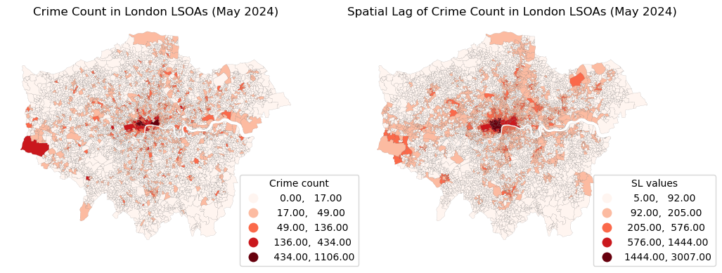
# Plot the original data and spatial lag of the crime data for comparison
fig, ax = plt.subplots(1, 2, figsize=(12, 6))
gdf_crime_agg_may.plot(column='Count', ax=ax[0], legend=True, cmap='Reds',
                       edgecolor='black', linewidth=0.05, scheme = 'naturalbreaks',
                       legend_kwds = {'bbox_to_anchor': (1.2, 0.35),'title': "Crime count"})
ax[0].set_title('Crime Count in London LSOAs (May 2024)')
gdf_crime_agg_may.plot(column='sl_Count', ax=ax[1], legend=True, cmap='Reds',
                       edgecolor='black', linewidth=0.05, scheme = 'naturalbreaks',
                       legend_kwds = {'bbox_to_anchor': (1.2, 0.35),'title': "SL values"})
ax[1].set_title('Spatial Lag of Crime Count in London LSOAs (May 2024)')
ax[0].set_axis_off()
ax[1].set_axis_off()
plt.show()
5.2 Spatial Lag Model (SLM)#
The Spatial Lag Model (SLM) is a type of regression model that explicitly includes the effect of neighboring dependent variable values (i.e., spatial lag) on the value at each location:
\(\mathbf{y}\) is the vector of the dependent variable
\(\mathbf{W}\) is the spatial weights matrix, so \(\mathbf{W y}\) is the spatial lag of \(\mathbf{y}\)
\(\rho\) is the spatial autoregressive coefficient
\(\mathbf{X}\) is the matrix of explanatory variables
\(\boldsymbol{\beta}\) is the vector of coefficients
\(\boldsymbol{\epsilon}\) is the error term
We need a new pkg called spreg as a part of libpysal to compute the spatial lag model. The columbus data frame has 49 rows and 22 columns. Unit of analysis: 49 neighbourhoods in Columbus, OH, 1980 data. The Spatial Lag Model documentation can be found here.
import spreg
from libpysal.examples import load_example
from spreg import ML_Lag  # Maximum Likelihood Spatial Lag Model
# Load sample dataset
data = load_example('Columbus')
gdf_columbus = gpd.read_file(data.get_path('columbus.shp'))
gdf_columbus.head()
| AREA | PERIMETER | COLUMBUS_ | COLUMBUS_I | POLYID | NEIG | HOVAL | INC | CRIME | OPEN | ... | DISCBD | X | Y | NSA | NSB | EW | CP | THOUS | NEIGNO | geometry | |
|---|---|---|---|---|---|---|---|---|---|---|---|---|---|---|---|---|---|---|---|---|---|
| 0 | 0.309441 | 2.440629 | 2 | 5 | 1 | 5 | 80.467003 | 19.531 | 15.725980 | 2.850747 | ... | 5.03 | 38.799999 | 44.070000 | 1.0 | 1.0 | 1.0 | 0.0 | 1000.0 | 1005.0 | POLYGON ((8.62413 14.23698, 8.5597 14.74245, 8... |
| 1 | 0.259329 | 2.236939 | 3 | 1 | 2 | 1 | 44.567001 | 21.232 | 18.801754 | 5.296720 | ... | 4.27 | 35.619999 | 42.380001 | 1.0 | 1.0 | 0.0 | 0.0 | 1000.0 | 1001.0 | POLYGON ((8.25279 14.23694, 8.28276 14.22994, ... |
| 2 | 0.192468 | 2.187547 | 4 | 6 | 3 | 6 | 26.350000 | 15.956 | 30.626781 | 4.534649 | ... | 3.89 | 39.820000 | 41.180000 | 1.0 | 1.0 | 1.0 | 0.0 | 1000.0 | 1006.0 | POLYGON ((8.65331 14.00809, 8.81814 14.00205, ... |
| 3 | 0.083841 | 1.427635 | 5 | 2 | 4 | 2 | 33.200001 | 4.477 | 32.387760 | 0.394427 | ... | 3.70 | 36.500000 | 40.520000 | 1.0 | 1.0 | 0.0 | 0.0 | 1000.0 | 1002.0 | POLYGON ((8.4595 13.82035, 8.47341 13.83227, 8... |
| 4 | 0.488888 | 2.997133 | 6 | 7 | 5 | 7 | 23.225000 | 11.252 | 50.731510 | 0.405664 | ... | 2.83 | 40.009998 | 38.000000 | 1.0 | 1.0 | 1.0 | 0.0 | 1000.0 | 1007.0 | POLYGON ((8.68527 13.63952, 8.67758 13.72221, ... |
5 rows × 21 columns
# we need to set the crs to EPSG:26917 (NAD83 / UTM zone 17N) as the polygon valus in the data is in this CRS, not the EPSG:4326.
gdf_columbus = gdf_columbus.set_crs(epsg=26917, allow_override=True)
print(gdf_columbus.crs)
EPSG:26917
gdf_columbus[['INC', 'HOVAL', 'CRIME']]
| INC | HOVAL | CRIME | |
|---|---|---|---|
| 0 | 19.531000 | 80.467003 | 15.725980 |
| 1 | 21.232000 | 44.567001 | 18.801754 |
| 2 | 15.956000 | 26.350000 | 30.626781 |
| 3 | 4.477000 | 33.200001 | 32.387760 |
| 4 | 11.252000 | 23.225000 | 50.731510 |
| 5 | 16.028999 | 28.750000 | 26.066658 |
| 6 | 8.438000 | 75.000000 | 0.178269 |
| 7 | 11.337000 | 37.125000 | 38.425858 |
| 8 | 17.586000 | 52.599998 | 30.515917 |
| 9 | 13.598000 | 96.400002 | 34.000835 |
| 10 | 7.467000 | 19.700001 | 62.275448 |
| 11 | 10.048000 | 19.900000 | 56.705669 |
| 12 | 9.549000 | 41.700001 | 46.716129 |
| 13 | 9.963000 | 42.900002 | 57.066132 |
| 14 | 9.873000 | 18.000000 | 48.585487 |
| 15 | 7.625000 | 18.799999 | 54.838711 |
| 16 | 9.798000 | 41.750000 | 36.868774 |
| 17 | 13.185000 | 60.000000 | 43.962486 |
| 18 | 11.618000 | 30.600000 | 54.521965 |
| 19 | 31.070000 | 81.266998 | 0.223797 |
| 20 | 10.655000 | 19.975000 | 40.074074 |
| 21 | 11.709000 | 30.450001 | 33.705048 |
| 22 | 21.155001 | 47.733002 | 20.048504 |
| 23 | 14.236000 | 53.200001 | 38.297871 |
| 24 | 8.461000 | 17.900000 | 61.299175 |
| 25 | 8.085000 | 20.299999 | 40.969742 |
| 26 | 10.822000 | 34.099998 | 52.794430 |
| 27 | 7.856000 | 22.850000 | 56.919785 |
| 28 | 8.681000 | 32.500000 | 60.750446 |
| 29 | 13.906000 | 22.500000 | 68.892044 |
| 30 | 16.940001 | 31.799999 | 17.677214 |
| 31 | 18.941999 | 40.299999 | 19.145592 |
| 32 | 9.918000 | 23.600000 | 41.968163 |
| 33 | 14.948000 | 28.450001 | 23.974028 |
| 34 | 12.814000 | 27.000000 | 39.175053 |
| 35 | 18.739000 | 36.299999 | 14.305556 |
| 36 | 17.017000 | 43.299999 | 42.445076 |
| 37 | 11.107000 | 22.700001 | 53.710938 |
| 38 | 18.476999 | 39.599998 | 19.100863 |
| 39 | 29.833000 | 61.950001 | 16.241299 |
| 40 | 22.207001 | 42.099998 | 18.905146 |
| 41 | 25.872999 | 44.333000 | 16.491890 |
| 42 | 13.380000 | 25.700001 | 36.663612 |
| 43 | 16.961000 | 33.500000 | 25.962263 |
| 44 | 14.135000 | 27.733000 | 29.028488 |
| 45 | 18.323999 | 76.099998 | 16.530533 |
| 46 | 18.950001 | 42.500000 | 27.822861 |
| 47 | 11.813000 | 26.799999 | 26.645266 |
| 48 | 18.796000 | 35.799999 | 22.541491 |
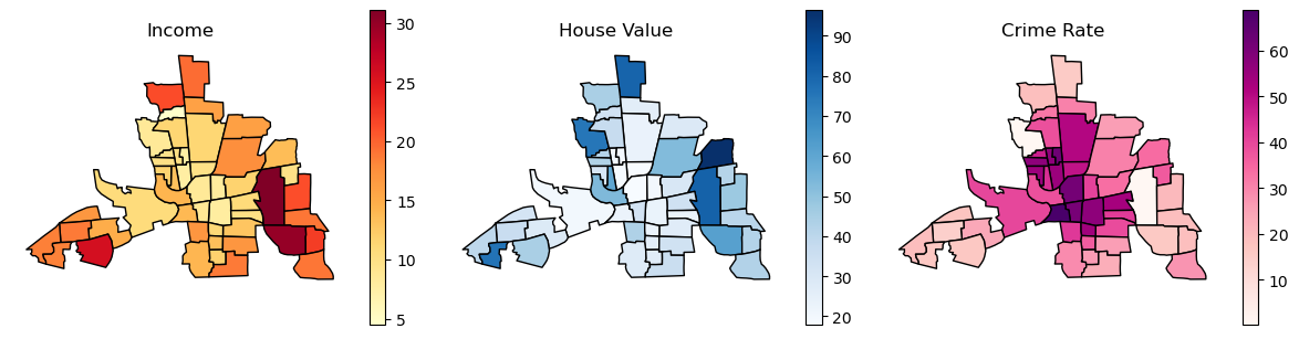
# plot the three maps of the columbus data: income ('INC'), house value ('HOVAL') and crime rate ('CRIME')
fig, ax = plt.subplots(1, 3, figsize=(12, 6))
gdf_columbus.plot(column='INC', ax=ax[0], legend=True, cmap='YlOrRd', edgecolor='black', legend_kwds={'shrink': 0.5})
ax[0].set_title('Income')
ax[0].axis('off')
gdf_columbus.plot(column='HOVAL', ax=ax[1], legend=True, cmap='Blues', edgecolor='black', legend_kwds={'shrink': 0.5})
ax[1].set_title('House Value')
ax[1].axis('off')
gdf_columbus.plot(column='CRIME', ax=ax[2], legend=True, cmap='RdPu', edgecolor='black', legend_kwds={'shrink': 0.5})
ax[2].set_title('Crime Rate')
ax[2].axis('off')
plt.tight_layout()
# Spatial weights
w = weights.Queen.from_dataframe(gdf_columbus, use_index='True')
w.transform = 'R'  # Row-standardized

# Variables
y = gdf_columbus[['CRIME']].values          # Dependent variable / matrix
X = gdf_columbus[['INC', 'HOVAL']].values   # Independent variables are Income and House Value.
# Fit spatial lag model
model_sl = ML_Lag(y, X, w=w, name_y='CRIME', name_x=['INC', 'HOVAL'], name_w='Queen', name_ds='Columbus')

# Output summary
print(model_sl.summary)
REGRESSION RESULTS
------------------

SUMMARY OF OUTPUT: MAXIMUM LIKELIHOOD SPATIAL LAG (METHOD = FULL)
-----------------------------------------------------------------
Data set            :    Columbus
Weights matrix      :       Queen
Dependent Variable  :       CRIME                Number of Observations:          49
Mean dependent var  :     35.1288                Number of Variables   :           4
S.D. dependent var  :     16.7321                Degrees of Freedom    :          45
Pseudo R-squared    :      0.6473
Spatial Pseudo R-squared:  0.5806
Log likelihood      :   -182.6740
Sigma-square ML     :     96.8572                Akaike info criterion :     373.348
S.E of regression   :      9.8416                Schwarz criterion     :     380.915

------------------------------------------------------------------------------------
            Variable     Coefficient       Std.Error     z-Statistic     Probability
------------------------------------------------------------------------------------
            CONSTANT        45.60325         7.25740         6.28369         0.00000
                 INC        -1.04873         0.30741        -3.41154         0.00065
               HOVAL        -0.26633         0.08910        -2.98929         0.00280
             W_CRIME         0.42333         0.11951         3.54216         0.00040
------------------------------------------------------------------------------------

SPATIAL LAG MODEL IMPACTS
Impacts computed using the 'simple' method.
            Variable         Direct        Indirect          Total
                 INC        -1.0487         -0.7699         -1.8186
               HOVAL        -0.2663         -0.1955         -0.4618
================================ END OF REPORT =====================================
Interpretation of the results:
Number of Variables: Includes intercept/constant, two predictors /independent variables(
INC,HOVAL), and spatial lag \(y\) (the spatial lag is inherently calculated as part of the model fitting process) (W_CRIME);Pseudo \(R^2\): Indicates Goodness of model fit (similar to \(R^2\) in OLS), here, ~65% of variance explained (higher is better);
Spatial Pseudo \(R^2\): Fit due to the spatial component (higher is better);
Sigma-square ML: Maximum likelihood estimate of error variance;
Standard Error of Regression: Residual spread;
Log Likelihood: Used for model comparison (higher is better);
AIC/ Akaike Information Criterion: Used for model comparison (lower is better);
Schwarz Criterion (BIC): Bayesian Information Criterion (penalizes model complexity) (Lower BIC is better);
The coefficient of variable: it reflects the relationship between each independent variable and the dependent variable. A positive coefficient means the variable is positively correlated with the dependent variable — as the independent variable increases, the dependent variable tends to increase. A negative coefficient means the variable is negatively correlated — as the independent variable increases, the dependent variable tends to decrease.
The z-statistic (also called the Wald statistic) tests whether a coefficient is significantly different from zero. A high absolute z-value (e.g., > 2 or < -2) suggests the coefficient is statistically significant.
The p-value tells you the probability of observing a coefficient as extreme as the one calculated, assuming the true coefficient is zero (i.e., null hypothesis is true). Low p-values (< 0.05) -> reject the null hypothesis -> the variable is significant. High p-values (> 0.05) -> fail to reject the null -> variable may not be important.
In summary, the results reflect the spatial lag model equation, where the spatial autoregressive coefficient \(\rho\) corresponds to the coefficient of W_CRIME (0.42). The vector of regression coefficients \(\boldsymbol{\beta}\) includes the coefficients for INC and HOVAL, which are -1.05 and -0.27 respectively. The error term \(\boldsymbol{\epsilon}\) is represented by the standard error of the regression (9.84) and the maximum likelihood estimate of the error variance (Sigma-square ML = 96.86).
Residuals analysis
If residuals still show spatial autocorrelation –> model may be misspecified. In other words, it suggests that your model isn’t fully capturing the spatial structure in the data.
residuals = model_sl.u  # residuals from the SLM
moran_resid = esda.Moran(residuals, w)
print(moran_resid.I, moran_resid.p_sim)
0.03306830572737454 0.258
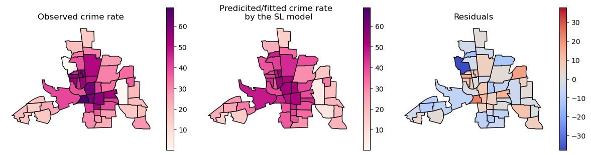
We can also plot the fitted y values and residuals/errors in residuals analysis:
Mapping fitted values: show where your model thinks the crime rate is high/low.
Mapping residual values: show where the model over/underpredicting.
# get the in sample prediction (fitted) crime rates and the residuals
gdf_columbus["fitted"] = model_sl.predy.flatten()
gdf_columbus["residuals"] = model_sl.u.flatten()
fig, ax = plt.subplots(1, 3, figsize=(12, 6))
gdf_columbus.plot(column='CRIME', ax=ax[0], legend=True, cmap='RdPu', edgecolor='black', legend_kwds={'shrink': 0.5},
                  vmin=gdf_columbus.CRIME.min(), vmax=gdf_columbus.CRIME.max())
ax[0].set_title('Observed crime rate')
ax[0].axis('off')
gdf_columbus.plot(column='fitted', ax=ax[1], legend=True, cmap='RdPu', edgecolor='black', legend_kwds={'shrink': 0.5}, vmin=gdf_columbus.CRIME.min(), vmax=gdf_columbus.CRIME.max())
ax[1].set_title('Predicited/fitted crime rate \n by the SL model')
ax[1].axis('off')
gdf_columbus.plot(column='residuals', ax=ax[2], legend=True, cmap='coolwarm', edgecolor='black', legend_kwds={'shrink': 0.5},
                  vmin=gdf_columbus.residuals.min(), vmax=abs(gdf_columbus.residuals.min()))
ax[2].set_title('Residuals')
ax[2].axis('off')
plt.tight_layout()
5.3 Spatial Error Model (SEM)#
The Spatial Error Model (SEM) accounts for spatial autocorrelation in regression error terms. It is used when spatially correlated unobserved variables that affect the dependent variable are omitted from the model. Rather than directly impacting the dependent variable, spatial effects are captured within the error terms themselves.
The Spatial Error Model (SEM) is given by:
where:
\(\mathbf{y}\) is the dependent variable,
\(\mathbf{X}\) is the matrix of independent variables,
\(\boldsymbol{\beta}\) is the vector of coefficients,
\(\mathbf{u}\) is the error term.
The error term is spatially correlated, and can be expressed as:
where:
\(\lambda\) is the spatial autoregressive parameter,
\(\mathbf{W}\) is the spatial weight matrix,
\(\boldsymbol{\epsilon}\) is the white noise error term.
Thus, the SEM model is:
from spreg import ML_Error  # Maximum Likelihood Spatial Error Model
# Use the same X and y variables in gdf_columbus
# Fit the spatial error model
model_sem = ML_Error(y, X, w=w, name_y='CRIME', name_x=['INC', 'HOVAL'], name_w='Queen', name_ds='Columbus')
# Output summary
print(model_sem.summary)
REGRESSION RESULTS
------------------

SUMMARY OF OUTPUT: ML SPATIAL ERROR (METHOD = full)
---------------------------------------------------
Data set            :    Columbus
Weights matrix      :       Queen
Dependent Variable  :       CRIME                Number of Observations:          49
Mean dependent var  :     35.1288                Number of Variables   :           3
S.D. dependent var  :     16.7321                Degrees of Freedom    :          46
Pseudo R-squared    :      0.5362
Log likelihood      :   -183.7494
Sigma-square ML     :     97.6742                Akaike info criterion :     373.499
S.E of regression   :      9.8830                Schwarz criterion     :     379.174

------------------------------------------------------------------------------------
            Variable     Coefficient       Std.Error     z-Statistic     Probability
------------------------------------------------------------------------------------
            CONSTANT        60.27947         5.36559        11.23444         0.00000
                 INC        -0.95731         0.33423        -2.86420         0.00418
               HOVAL        -0.30456         0.09205        -3.30873         0.00094
              lambda         0.54675         0.13805         3.96052         0.00007
------------------------------------------------------------------------------------
================================ END OF REPORT =====================================
Interpretation:
For model comparison, the Spatial Lag Model (SL) demonstrates better performance than the Spatial Error Model (SE), as indicated by its higher R² and log-likelihood values. Although the AIC values for SL are only slightly better than SE, the difference is not substantial enough to definitively favor one model based solely on these criteria.
5.4 Spatial Durbin Model (SDM)#
The Spatial Durbin Model (SDM) extends the spatial lag model (SAR) by including spatially lagged independent variables in addition to the spatially lagged dependent variable. It allows for capturing spatial dependence in both the dependent and independent variables.
The Spatial Durbin Model (SDM) is specified as:
where:
\( \mathbf{y} \) is the dependent variable vector,
\( \rho \mathbf{W} \mathbf{y} \) represents the spatial lag of the dependent variable,
\( \mathbf{X} \boldsymbol{\beta} \) are the usual covariates,
\( \mathbf{W} \mathbf{X} \boldsymbol{\theta} \) are the spatially lagged covariates,
\( \boldsymbol{\varepsilon} \sim \mathcal{N}(0, \sigma^2 \mathbf{I}) \) is the error term.
We also use the function spreg.ML_Lag but need to set the parameter slx_lags(Number of spatial lags of X to include in the model specification. If slx_lags>0, the specification becomes of the Spatial Durbin type) and slx_var (either All(default) or list of booleans to select x variables to be lagged)
# Fit spatial durbin model
model_dur = ML_Lag(y, X, w=w, name_y='CRIME', name_x=['INC', 'HOVAL'], name_w='Queen', name_ds='Columbus', slx_lags=1)

# Output summary
print(model_dur.summary)
REGRESSION RESULTS
------------------

SUMMARY OF OUTPUT: MAXIMUM LIKELIHOOD SPATIAL LAG WITH SLX - SPATIAL DURBIN MODEL (METHOD = FULL)
-------------------------------------------------------------------------------------------------
Data set            :    Columbus
Weights matrix      :       Queen
Dependent Variable  :       CRIME                Number of Observations:          49
Mean dependent var  :     35.1288                Number of Variables   :           6
S.D. dependent var  :     16.7321                Degrees of Freedom    :          43
Pseudo R-squared    :      0.6603
Spatial Pseudo R-squared:  0.6120
Log likelihood      :   -181.6393
Sigma-square ML     :     93.2722                Akaike info criterion :     375.279
S.E of regression   :      9.6578                Schwarz criterion     :     386.629

------------------------------------------------------------------------------------
            Variable     Coefficient       Std.Error     z-Statistic     Probability
------------------------------------------------------------------------------------
            CONSTANT        44.32001        13.04547         3.39735         0.00068
                 INC        -0.91991         0.33474        -2.74811         0.00599
               HOVAL        -0.29713         0.09042        -3.28625         0.00102
               W_INC        -0.58391         0.57422        -1.01687         0.30921
             W_HOVAL         0.25768         0.18723         1.37626         0.16874
             W_CRIME         0.40346         0.16133         2.50079         0.01239
------------------------------------------------------------------------------------

DIAGNOSTICS FOR SPATIAL DEPENDENCE
TEST                              DF         VALUE           PROB
Common Factor Hypothesis Test     2          4.474           0.1068

SPATIAL DURBIN MODEL IMPACTS
Impacts computed using the 'simple' method.
            Variable         Direct        Indirect          Total
                 INC        -0.9199         -1.6010         -2.5209
               HOVAL        -0.2971          0.2310         -0.0661
================================ END OF REPORT =====================================
Interpretation:
Based on the results of the report, we can observe that the Spatial Durbin Model (SDM) fits the data using a different approach. Firstly, we notice that the spatial lag variables of the independent variables — specifically, W_INC and W_HOVAL — have p-values greater than 0.05, indicating that they are not statistically significant. However, when considering metrics such as \(R^2\) and log likelihood, the SDM shows slightly better performance compared to the Spatial Lag Model (SLM) and the Spatial Error Model (SEM) which suggest a marginally stronger overall fit.
5.5 Geographically Weighted Regression (GWR)#
Geographically Weighted Regression (GWR) is an extension of traditional regression that allows the relationships between independent variables (X) and the dependent variable (y) to vary across geographic space.
The linear regression /OLS:
GWR:
Where:
\( y_i \): Dependent variable / Response variable at location \( i \);
\( x_{ik} \): \( k -th\) independent variable/predictor at location \( i \);
\( (u_i, v_i) \): Coordinates of location \( i \);
\( \beta_k(u_i, v_i) \): Location-specific regression coefficient for variable \( k \) at location \(i\);
\( \varepsilon_i \): Error term;
\( n \) is the number of observations;
\( p \) is the number of independent variables;
\(\beta_0\) is the intercept.
Weighted Least Squares Estimation
Each local coefficient \( \hat{\boldsymbol{\beta}}(u_i, v_i) \) is estimated by solving:
Where:
\( X \): Matrix of predictors/ dependent variables/ features;
\( W_i \): Spatial weighting matrix for location \( i \);
\( \boldsymbol{y} \): Vector of observed responses.
Kernel Function for Weights (e.g., Gaussian)
Where:
\( d_{ij} \): Distance between location \( i \) and \( j \)
\( b \): Bandwidth parameter
Example: Calculating the local coefficient \( \hat{\boldsymbol{\beta}}(u_0, v_0)\)
data
index \(i,j\) |
\(x\) |
\(y\) |
\(u (lon)\) |
\(v (lat)\) |
|---|---|---|---|---|
1 |
1.0 |
2.0 |
0.0 |
0.0 |
2 |
2.0 |
3.0 |
1.0 |
0.0 |
3 |
3.0 |
6.0 |
0.0 |
1.0 |
4 |
4.0 |
8.0 |
1.0 |
1.0 |
Fitting the equation of GWR:
Calculating dist
index \(i\) |
Coords |
Dist to (0, 0) |
|---|---|---|
1 |
(0, 0) |
0.00 |
2 |
(1, 0) |
1.00 |
3 |
(0, 1) |
1.00 |
4 |
(1, 1) |
1.41 |
Calculating spatial weight (set bandwith = 1) using
\(w_{j} = \exp\left( -\frac{d_{j}^2}{1} \right)\),
Exponential function: \(\exp(x) = e^x\) (\(e\) is Euler’s number, approximately 2.71828)
index \(i,j\) |
Dis \(d_j\) to i (0,0) |
Spatial weight \(w_1j\) |
|---|---|---|
1 |
0.00 |
1.00 |
2 |
1.00 |
0.37 |
3 |
1.00 |
0.37 |
4 |
1.41 |
0.14 |
Caculating the local coefficent vector:
The \(\mathbf{X} \) and vector \( \mathbf{y}\) are:
Calculating the diagonal matrix:
- \[\begin{split}\mathbf{X}^T \mathbf{W} \mathbf{X} = \begin{bmatrix} 1 & 1 & 1 & 1 \\ 1 & 2 & 3 & 4 \end{bmatrix} \cdot \begin{bmatrix} 1.0 & 0 & 0 & 0 \\ 0 & 0.37 & 0 & 0 \\ 0 & 0 & 0.37 & 0 \\ 0 & 0 & 0 & 0.14 \end{bmatrix} \cdot \begin{bmatrix} 1 & 1 \\ 1 & 2 \\ 1 & 3 \\ 1 & 4 \end{bmatrix} = \begin{bmatrix} 1.88 & 3.41 \\ 3.41 & 8.05 \end{bmatrix} \end{split}\]
- \[\begin{split} \mathbf{X}^T \mathbf{W} \mathbf{y} = \begin{bmatrix} 1 & 1 & 1 & 1 \\ 1 & 2 & 3 & 4 \end{bmatrix} \cdot \begin{bmatrix} 1.0 & 0 & 0 & 0 \\ 0 & 0.37 & 0 & 0 \\ 0 & 0 & 0.37 & 0 \\ 0 & 0 & 0 & 0.14 \end{bmatrix} \cdot \begin{bmatrix} 2 \\ 3 \\ 6\\ 8 \end{bmatrix} = \begin{bmatrix} 6.45 \\ 15.36 \end{bmatrix}\end{split}\]
- \[\begin{split} \hat{\boldsymbol{\beta}}(u_0, v_0) = \left( X^\top W X \right)^{-1} X^\top W \boldsymbol{y} = (\begin{bmatrix} 1.88 & 3.41 \\ 3.41 & 8.05 \end{bmatrix})^{-1} \cdot \begin{bmatrix} 6.45 \\ 15.36 \end{bmatrix} = \begin{bmatrix} -0.13 \\ 1.96 \end{bmatrix}\end{split}\]
# an example to calculate the expotional function
import math
print(math.exp(0),
      math.exp(-1),
      math.exp(-1),
      math.exp(-(1.41*1.41)))
1.0 0.36787944117144233 0.36787944117144233 0.13695539364545323
# Calculating the diagonal matrix
W = np.diag([1, 0.3679, 0.3679, 0.1370])
print(W)
[[1.     0.     0.     0.    ]
 [0.     0.3679 0.     0.    ]
 [0.     0.     0.3679 0.    ]
 [0.     0.     0.     0.137 ]]
# set X and y
X = np.array([
    [1, 1],
    [1, 2],
    [1, 3],
    [1, 4]
])
y = np.array([2, 3, 6, 8])
#  Spatial weights matrix W
weights = np.array([1.0, 0.37, 0.37, 0.14])
W = np.diag(weights)
# Calculate XT W X
XTWX = X.T @ W @ X
# Calculate XT W y
XTWy = X.T @ W @ y
# Calculate local coefficients beta_hat
beta_hat = np.linalg.inv(XTWX) @ XTWy
print("XTWX:\n", XTWX)
print("XTWy:\n", XTWy)
print("Estimated local coefficients beta_hat:\n", beta_hat)
XTWX:
 [[1.88 3.41]
 [3.41 8.05]]
XTWy:
 [ 6.45 15.36]
Estimated local coefficients beta_hat:
 [-0.12980975  1.96306227]
As a part of PySAL community, mgwr provide the GWR and mGWR model in python.
from mgwr.gwr import GWR, MGWR
from mgwr.sel_bw import Sel_BW
print(np.__version__)
1.26.4
We use Homicides and selected socio-economic characteristics for continental U.S. counties as an example for gwr and mgwr. Data for four decennial census years: 1960, 1970, 1980 and 1990.
import libpysal
us_hse = libpysal.examples.load_example("NCOVR")
gdf_us_hse = gpd.read_file(us_hse.get_path('NAT.shp'))
gdf_us_hse = gdf_us_hse.to_crs("EPSG:5070")
gdf_us_hse
| NAME | STATE_NAME | STATE_FIPS | CNTY_FIPS | FIPS | STFIPS | COFIPS | FIPSNO | SOUTH | HR60 | ... | BLK90 | GI59 | GI69 | GI79 | GI89 | FH60 | FH70 | FH80 | FH90 | geometry | |
|---|---|---|---|---|---|---|---|---|---|---|---|---|---|---|---|---|---|---|---|---|---|
| 0 | Lake of the Woods | Minnesota | 27 | 077 | 27077 | 27 | 77 | 27077 | 0 | 0.000000 | ... | 0.024534 | 0.285235 | 0.372336 | 0.342104 | 0.336455 | 11.279621 | 5.400000 | 5.663881 | 9.515860 | POLYGON ((49050.745 2838555.999, 49054.346 285... |
| 1 | Ferry | Washington | 53 | 019 | 53019 | 53 | 19 | 53019 | 0 | 0.000000 | ... | 0.317712 | 0.256158 | 0.360665 | 0.361928 | 0.360640 | 10.053476 | 2.600000 | 10.079576 | 11.397059 | POLYGON ((-1704187.741 2978490.561, -1690089.6... |
| 2 | Stevens | Washington | 53 | 065 | 53065 | 53 | 65 | 53065 | 0 | 1.863863 | ... | 0.210030 | 0.283999 | 0.394083 | 0.357566 | 0.369942 | 9.258437 | 5.600000 | 6.812127 | 10.352015 | POLYGON ((-1598348.829 2964085.947, -1605943.0... |
| 3 | Okanogan | Washington | 53 | 047 | 53047 | 53 | 47 | 53047 | 0 | 2.612330 | ... | 0.155922 | 0.258540 | 0.371218 | 0.381240 | 0.394519 | 9.039900 | 8.100000 | 10.084926 | 12.840340 | POLYGON ((-1713271.344 2979541.451, -1712880.7... |
| 4 | Pend Oreille | Washington | 53 | 051 | 53051 | 53 | 51 | 53051 | 0 | 0.000000 | ... | 0.134605 | 0.243263 | 0.365614 | 0.358706 | 0.387848 | 8.243930 | 4.100000 | 7.557643 | 10.313002 | POLYGON ((-1574802.183 3066600.159, -1545432.6... |
| ... | ... | ... | ... | ... | ... | ... | ... | ... | ... | ... | ... | ... | ... | ... | ... | ... | ... | ... | ... | ... | ... |
| 3080 | La Paz | Arizona | 04 | 012 | 04012 | 4 | 12 | 4012 | 0 | 5.046682 | ... | 2.628811 | 0.271556 | 0.364110 | 0.372662 | 0.405743 | 9.216414 | 8.000000 | 9.296093 | 12.379134 | POLYGON ((-1708456.819 1273380.859, -1711763.0... |
| 3081 | Cibola | New Mexico | 35 | 006 | 35006 | 35 | 6 | 35006 | 0 | 3.411368 | ... | 1.001029 | 0.287346 | 0.347426 | 0.363889 | 0.404823 | 9.645881 | 9.300000 | 11.925297 | 14.907666 | POLYGON ((-1016458.583 1340151.199, -1063696.6... |
| 3082 | York | Virginia | 51 | 199 | 51199 | 51 | 199 | 51199 | 1 | 1.544425 | ... | 12.534861 | 0.271201 | 0.279962 | 0.310047 | 0.326229 | 8.776244 | 6.300000 | 8.063281 | 9.825284 | POLYGON ((1713621.948 1740205.362, 1713411.118... |
| 3083 | Prince William | Virginia | 51 | 153 | 51153 | 51 | 153 | 51153 | 1 | 9.302820 | ... | 11.365661 | 0.240268 | 0.288488 | 0.289718 | 0.286416 | 7.525717 | 5.300000 | 8.626065 | 10.276895 | POLYGON ((1584066.804 1880564.938, 1562143.846... |
| 3084 | Gallatin | Montana | 30 | 031 | 30031 | 30 | 31 | 30031 | 0 | 3.396162 | ... | 0.228960 | 0.245227 | 0.343359 | 0.344086 | 0.377684 | 8.598461 | 5.651882 | 8.166075 | 10.187915 | POLYGON ((-1209699.354 2515401.971, -1198622.3... |
3085 rows × 70 columns
gdf_us_hse.columns
Index(['NAME', 'STATE_NAME', 'STATE_FIPS', 'CNTY_FIPS', 'FIPS', 'STFIPS',
       'COFIPS', 'FIPSNO', 'SOUTH', 'HR60', 'HR70', 'HR80', 'HR90', 'HC60',
       'HC70', 'HC80', 'HC90', 'PO60', 'PO70', 'PO80', 'PO90', 'RD60', 'RD70',
       'RD80', 'RD90', 'PS60', 'PS70', 'PS80', 'PS90', 'UE60', 'UE70', 'UE80',
       'UE90', 'DV60', 'DV70', 'DV80', 'DV90', 'MA60', 'MA70', 'MA80', 'MA90',
       'POL60', 'POL70', 'POL80', 'POL90', 'DNL60', 'DNL70', 'DNL80', 'DNL90',
       'MFIL59', 'MFIL69', 'MFIL79', 'MFIL89', 'FP59', 'FP69', 'FP79', 'FP89',
       'BLK60', 'BLK70', 'BLK80', 'BLK90', 'GI59', 'GI69', 'GI79', 'GI89',
       'FH60', 'FH70', 'FH80', 'FH90', 'geometry'],
      dtype='object')
For independent variables, we use ‘UE90’, ‘POL90’, ‘GI89’ which refer to the Unemployment rate, Resource deprivation and Gini index of family income inequality of 1990; the dependent variable is ‘HR90’, i.e., Homicide rate per 100,000
gdf_us_hse[['HR90', 'UE90', 'RD90', 'GI89']]
| HR90 | UE90 | RD90 | GI89 | |
|---|---|---|---|---|
| 0 | 0.000000 | 3.894790 | -0.802774 | 0.336455 |
| 1 | 15.885624 | 16.811594 | -0.135483 | 0.360640 |
| 2 | 6.462453 | 10.700794 | -0.276544 | 0.369942 |
| 3 | 6.996502 | 10.203544 | 0.370762 | 0.394519 |
| 4 | 7.478033 | 14.991023 | 0.107992 | 0.387848 |
| ... | ... | ... | ... | ... |
| 3080 | 5.521552 | 10.910351 | 0.494534 | 0.405743 |
| 3081 | 8.691999 | 11.002271 | 0.688425 | 0.404823 |
| 3082 | 4.367330 | 4.102888 | -1.339770 | 0.326229 |
| 3083 | 3.727712 | 3.353981 | -1.747367 | 0.286416 |
| 3084 | 2.048855 | 5.488553 | -0.361145 | 0.377684 |
3085 rows × 4 columns
from mgwr.gwr import GWR
from mgwr.sel_bw import Sel_BW
import warnings
warnings.filterwarnings('ignore')

# Ensure geometries are projected (e.g., EPSG:5070)
gdf_us_hse = gdf_us_hse.to_crs(epsg=5070)

# Extract centroids and coordinates
centroids = gdf_us_hse.geometry.centroid
coords = pd.DataFrame({
    'X': centroids.x,
    'Y': centroids.y}).values

# Dependent and independent variables
y= gdf_us_hse[['HR90']].values
X= gdf_us_hse[['UE90', 'RD90', 'GI89']].values
# select bandwidth
bw_selector = Sel_BW(coords, y, X, kernel='gaussian')
bw = bw_selector.search(bw_min=20)
print(f"Optimal bandwidth: {bw}")
Optimal bandwidth: 26.0
# fit the gwr_model
gwr_model = GWR(coords, y, X, bw)
gwr_results = gwr_model.fit()
np.float = float # Monkey patch, as gwr.summary() relies on numpy version < 1.24
gwr_results.summary()
===========================================================================
Model type                                                         Gaussian
Number of observations:                                                3085
Number of covariates:                                                     4

Global Regression Results
---------------------------------------------------------------------------
Residual sum of squares:                                          89071.988
Log-likelihood:                                                   -9564.688
AIC:                                                              19137.376
AICc:                                                             19139.396
BIC:                                                              64318.288
R2:                                                                   0.345
Adj. R2:                                                              0.345

Variable                              Est.         SE  t(Est/SE)    p-value
------------------------------- ---------- ---------- ---------- ----------
X0                                  32.257      2.662     12.119      0.000
X1                                  -0.174      0.041     -4.274      0.000
X2                                   6.283      0.263     23.934      0.000
X3                                 -66.506      7.064     -9.415      0.000

Geographically Weighted Regression (GWR) Results
---------------------------------------------------------------------------
Spatial kernel:                                           Adaptive bisquare
Bandwidth used:                                                      26.000

Diagnostic information
---------------------------------------------------------------------------
Residual sum of squares:                                          34561.697
Effective number of parameters (trace(S)):                         1066.029
Degree of freedom (n - trace(S)):                                  2018.971
Sigma estimate:                                                       4.137
Log-likelihood:                                                   -8104.405
AIC:                                                              18342.868
AICc:                                                             19472.896
BIC:                                                              24781.647
R2:                                                                   0.746
Adjusted R2:                                                          0.612
Adj. alpha (95%):                                                     0.000
Adj. critical t value (95%):                                          3.740

Summary Statistics For GWR Parameter Estimates
---------------------------------------------------------------------------
Variable                   Mean        STD        Min     Median        Max
-------------------- ---------- ---------- ---------- ---------- ----------
X0                       25.316     61.088   -334.721     22.559    296.359
X1                       -0.069      1.135    -10.447     -0.042      6.231
X2                        4.520      7.703    -38.419      4.080     36.367
X3                      -48.895    153.210   -748.675    -45.006    866.587
===========================================================================
# Convert local R2 to df
localR2_df = pd.DataFrame(gwr_results.localR2, columns=["localR2"])
# Convert params to df
params_df = pd.DataFrame(gwr_results.params, columns=['intercept', 'UE90', 'RD90', 'GI89'])
# Convert t-statistic to df
tvalues_df = pd.DataFrame(gwr_results.tvalues, columns=['intercept_tv', 'UE90_tv', 'RD90_tv', 'GI89_tv'])

from scipy.stats import t
# Approximate degrees of freedom
free = gwr_results.n - gwr_results.k
# Compute approximate two-tailed p-values
pvalues = 2 * (1 - t.cdf(abs(gwr_results.tvalues), df=free))
pvalues_df = pd.DataFrame(pvalues, columns=['intercept_p', 'UE90_p', 'RD90_p', 'GI89_p'])

# Concat
df_m = pd.concat([localR2_df, params_df, tvalues_df, pvalues_df], axis=1)
df_m
| localR2 | intercept | UE90 | RD90 | GI89 | intercept_tv | UE90_tv | RD90_tv | GI89_tv | intercept_p | UE90_p | RD90_p | GI89_p | |
|---|---|---|---|---|---|---|---|---|---|---|---|---|---|
| 0 | 0.633629 | 29.324285 | -0.544060 | 8.825613 | -54.691183 | 0.530777 | -1.136838 | 1.206369 | -0.379389 | 0.595612 | 0.255694 | 2.277677e-01 | 0.704425 |
| 1 | 0.867377 | 39.572338 | 0.683470 | 6.282482 | -103.678889 | 0.523849 | 1.252162 | 0.661318 | -0.556264 | 0.600421 | 0.210606 | 5.084581e-01 | 0.578071 |
| 2 | 0.830943 | 19.896255 | 0.661203 | 4.685874 | -52.824834 | 0.328547 | 1.488115 | 0.596222 | -0.352140 | 0.742521 | 0.136823 | 5.510709e-01 | 0.724757 |
| 3 | 0.883899 | 69.724504 | 0.603537 | 8.337601 | -179.250594 | 0.836823 | 1.092445 | 0.775423 | -0.867623 | 0.402757 | 0.274723 | 4.381492e-01 | 0.385668 |
| 4 | 0.796476 | 3.273553 | 0.695606 | 2.205631 | -12.398164 | 0.059606 | 1.719729 | 0.308246 | -0.090220 | 0.952473 | 0.085582 | 7.579163e-01 | 0.928118 |
| ... | ... | ... | ... | ... | ... | ... | ... | ... | ... | ... | ... | ... | ... |
| 3080 | 0.254210 | 5.676060 | -0.319183 | -1.082073 | 15.286796 | 0.083111 | -0.382010 | -0.140611 | 0.088373 | 0.933769 | 0.702480 | 8.881867e-01 | 0.929586 |
| 3081 | 0.561805 | -30.728438 | 0.025356 | -1.208809 | 101.497956 | -0.709811 | 0.051656 | -0.215739 | 0.934326 | 0.477875 | 0.958806 | 8.292057e-01 | 0.350209 |
| 3082 | 0.412670 | -32.983666 | -1.603241 | -0.722064 | 138.316916 | -1.562146 | -2.494287 | -0.334925 | 2.340559 | 0.118356 | 0.012673 | 7.377043e-01 | 0.019318 |
| 3083 | 0.915385 | 135.867091 | 5.082617 | 20.600332 | -379.116343 | 4.149671 | 2.826873 | 5.045853 | -4.715368 | 0.000034 | 0.004731 | 4.776815e-07 | 0.000003 |
| 3084 | 0.396840 | -42.842168 | -0.435088 | -3.864959 | 127.061487 | -1.266138 | -0.884013 | -0.856698 | 1.428765 | 0.205559 | 0.376758 | 3.916784e-01 | 0.153173 |
3085 rows × 13 columns
gdf_us_co = gdf_us_hse[['NAME', 'STATE_NAME', 'geometry']]
gdf_us_co
| NAME | STATE_NAME | geometry | |
|---|---|---|---|
| 0 | Lake of the Woods | Minnesota | POLYGON ((49050.745 2838555.999, 49054.346 285... |
| 1 | Ferry | Washington | POLYGON ((-1704187.741 2978490.561, -1690089.6... |
| 2 | Stevens | Washington | POLYGON ((-1598348.829 2964085.947, -1605943.0... |
| 3 | Okanogan | Washington | POLYGON ((-1713271.344 2979541.451, -1712880.7... |
| 4 | Pend Oreille | Washington | POLYGON ((-1574802.183 3066600.159, -1545432.6... |
| ... | ... | ... | ... |
| 3080 | La Paz | Arizona | POLYGON ((-1708456.819 1273380.859, -1711763.0... |
| 3081 | Cibola | New Mexico | POLYGON ((-1016458.583 1340151.199, -1063696.6... |
| 3082 | York | Virginia | POLYGON ((1713621.948 1740205.362, 1713411.118... |
| 3083 | Prince William | Virginia | POLYGON ((1584066.804 1880564.938, 1562143.846... |
| 3084 | Gallatin | Montana | POLYGON ((-1209699.354 2515401.971, -1198622.3... |
3085 rows × 3 columns
gdf_us_co_gwr = pd.concat([gdf_us_co, df_m], axis=1)
gdf_us_co_gwr
| NAME | STATE_NAME | geometry | localR2 | intercept | UE90 | RD90 | GI89 | intercept_tv | UE90_tv | RD90_tv | GI89_tv | intercept_p | UE90_p | RD90_p | GI89_p | |
|---|---|---|---|---|---|---|---|---|---|---|---|---|---|---|---|---|
| 0 | Lake of the Woods | Minnesota | POLYGON ((49050.745 2838555.999, 49054.346 285... | 0.633629 | 29.324285 | -0.544060 | 8.825613 | -54.691183 | 0.530777 | -1.136838 | 1.206369 | -0.379389 | 0.595612 | 0.255694 | 2.277677e-01 | 0.704425 |
| 1 | Ferry | Washington | POLYGON ((-1704187.741 2978490.561, -1690089.6... | 0.867377 | 39.572338 | 0.683470 | 6.282482 | -103.678889 | 0.523849 | 1.252162 | 0.661318 | -0.556264 | 0.600421 | 0.210606 | 5.084581e-01 | 0.578071 |
| 2 | Stevens | Washington | POLYGON ((-1598348.829 2964085.947, -1605943.0... | 0.830943 | 19.896255 | 0.661203 | 4.685874 | -52.824834 | 0.328547 | 1.488115 | 0.596222 | -0.352140 | 0.742521 | 0.136823 | 5.510709e-01 | 0.724757 |
| 3 | Okanogan | Washington | POLYGON ((-1713271.344 2979541.451, -1712880.7... | 0.883899 | 69.724504 | 0.603537 | 8.337601 | -179.250594 | 0.836823 | 1.092445 | 0.775423 | -0.867623 | 0.402757 | 0.274723 | 4.381492e-01 | 0.385668 |
| 4 | Pend Oreille | Washington | POLYGON ((-1574802.183 3066600.159, -1545432.6... | 0.796476 | 3.273553 | 0.695606 | 2.205631 | -12.398164 | 0.059606 | 1.719729 | 0.308246 | -0.090220 | 0.952473 | 0.085582 | 7.579163e-01 | 0.928118 |
| ... | ... | ... | ... | ... | ... | ... | ... | ... | ... | ... | ... | ... | ... | ... | ... | ... |
| 3080 | La Paz | Arizona | POLYGON ((-1708456.819 1273380.859, -1711763.0... | 0.254210 | 5.676060 | -0.319183 | -1.082073 | 15.286796 | 0.083111 | -0.382010 | -0.140611 | 0.088373 | 0.933769 | 0.702480 | 8.881867e-01 | 0.929586 |
| 3081 | Cibola | New Mexico | POLYGON ((-1016458.583 1340151.199, -1063696.6... | 0.561805 | -30.728438 | 0.025356 | -1.208809 | 101.497956 | -0.709811 | 0.051656 | -0.215739 | 0.934326 | 0.477875 | 0.958806 | 8.292057e-01 | 0.350209 |
| 3082 | York | Virginia | POLYGON ((1713621.948 1740205.362, 1713411.118... | 0.412670 | -32.983666 | -1.603241 | -0.722064 | 138.316916 | -1.562146 | -2.494287 | -0.334925 | 2.340559 | 0.118356 | 0.012673 | 7.377043e-01 | 0.019318 |
| 3083 | Prince William | Virginia | POLYGON ((1584066.804 1880564.938, 1562143.846... | 0.915385 | 135.867091 | 5.082617 | 20.600332 | -379.116343 | 4.149671 | 2.826873 | 5.045853 | -4.715368 | 0.000034 | 0.004731 | 4.776815e-07 | 0.000003 |
| 3084 | Gallatin | Montana | POLYGON ((-1209699.354 2515401.971, -1198622.3... | 0.396840 | -42.842168 | -0.435088 | -3.864959 | 127.061487 | -1.266138 | -0.884013 | -0.856698 | 1.428765 | 0.205559 | 0.376758 | 3.916784e-01 | 0.153173 |
3085 rows × 16 columns
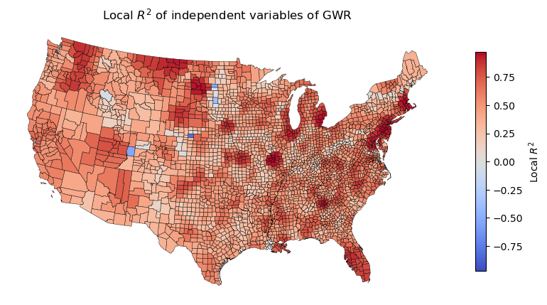
fig, ax = plt.subplots(figsize=(10, 8))
gdf_us_co_gwr.plot(ax=ax, column='localR2', cmap='coolwarm',
                   edgecolor='black',linewidth=0.3, legend=True, vmin=-max(gdf_us_co_gwr.localR2), vmax=max(gdf_us_co_gwr.localR2),
                   legend_kwds={'shrink': 0.5, 'orientation': 'vertical', 'label': 'Local $R^2$'})
ax.set_title('Local $R^2$ of independent variables of GWR' )
ax.axis('off')
plt.show()
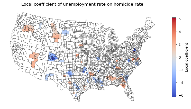
# plot the local coefficient
fig, ax = plt.subplots(figsize=(10, 8))

gdf_us_co_gwr[gdf_us_co_gwr['UE90_p'] < 0.05].plot(ax=ax, column='UE90',
                                                                    cmap='coolwarm', edgecolor='black',
                                                                    linewidth=0.3, legend=True,
                                                                    vmin=-max(gdf_us_co_gwr.UE90), vmax=max(gdf_us_co_gwr.UE90),
                                                                    legend_kwds={'shrink': 0.5, 'orientation': 'vertical', 'label': 'Local coefficient'})
# plot the not significant areas
gdf_us_co_gwr[gdf_us_co_gwr['UE90_p'] >= 0.05].plot(ax=ax, color='white', edgecolor='black', linewidth=0.3)
ax.set_title('Local coefficient of unemployment rate on homicide rate')
ax.axis('off')
plt.show()
5.6 Multiscale Geographically Weighted Regression (MGWR)#
MGWR (multiscale modelling) extends the GWR by allowing each predictor variable to operate at its own spatial scale (i.e., one \(bw_k\) per variable).
At spatial location \( i \), the MGWR model is expressed as:
\( y_i \): Dependent variable at location \( i \);
\( x_{ik} \): \( k^{th} \) independent variable at location \( i \);
\( \beta_k(bw_k, u_i, v_i) \): Spatially varying coefficient for variable \( k \);
\( bw_k \): Bandwidth specific to variable \( k \);
\( (u_i, v_i) \): Coordinates of location \( i \);
\( \varepsilon_i \): Error term.
In MGWR, each coefficient is estimated independently using its own kernel scale for variable-specific spatial smoothing:
Each variable \( x_k \) has its own bandwidth \( bw_k \).
A separate weight matrix \( W_k(u_i, v_i) \) is used for estimating the coefficient \( \beta_k \) at location \( i \).
# Extract centroids and coordinates
centroids = gdf_columbus.geometry.centroid
coords = pd.DataFrame({
    'X': centroids.x,
    'Y': centroids.y}).values

y = gdf_columbus[['CRIME']].values          # Dependent variable
X = gdf_columbus[['INC', 'HOVAL']].values   # Independent variables are Income and House Value.
GWR model
# select bandwidth
bw_selector = Sel_BW(coords, y, X, kernel='gaussian')
bw = bw_selector.search(bw_min=2)
print(f"Optimal bandwidth: {bw}")
Optimal bandwidth: 8.0
# fit the gwr_model
gwr_model = GWR(coords, y, X, bw)
gwr_results = gwr_model.fit()
np.float = float # Monkey patch, as gwr.summary() relies on numpy version < 1.24
gwr_results.summary()
===========================================================================
Model type                                                         Gaussian
Number of observations:                                                  49
Number of covariates:                                                     3

Global Regression Results
---------------------------------------------------------------------------
Residual sum of squares:                                           6014.893
Log-likelihood:                                                    -187.377
AIC:                                                                380.754
AICc:                                                               383.664
BIC:                                                               5835.869
R2:                                                                   0.552
Adj. R2:                                                              0.533

Variable                              Est.         SE  t(Est/SE)    p-value
------------------------------- ---------- ---------- ---------- ----------
X0                                  68.619      4.735     14.490      0.000
X1                                  -1.597      0.334     -4.780      0.000
X2                                  -0.274      0.103     -2.654      0.008

Geographically Weighted Regression (GWR) Results
---------------------------------------------------------------------------
Spatial kernel:                                           Adaptive bisquare
Bandwidth used:                                                       8.000

Diagnostic information
---------------------------------------------------------------------------
Residual sum of squares:                                            438.121
Effective number of parameters (trace(S)):                           33.760
Degree of freedom (n - trace(S)):                                    15.240
Sigma estimate:                                                       5.362
Log-likelihood:                                                    -123.200
AIC:                                                                315.919
AICc:                                                               503.685
BIC:                                                                381.679
R2:                                                                   0.967
Adjusted R2:                                                          0.890
Adj. alpha (95%):                                                     0.004
Adj. critical t value (95%):                                          2.986

Summary Statistics For GWR Parameter Estimates
---------------------------------------------------------------------------
Variable                   Mean        STD        Min     Median        Max
-------------------- ---------- ---------- ---------- ---------- ----------
X0                       61.120     16.533     29.348     61.983     97.408
X1                       -1.277      1.946     -7.292     -1.039      4.073
X2                       -0.204      0.927     -3.809     -0.113      1.963
===========================================================================
MGWR model
# Bandwidth selection
selector = Sel_BW(coords, y, X, multi=True)
bw = selector.search(bw_min=[2])
print(bw)
[44. 48. 44.]
# Fit MGWR model
mgwr_model = MGWR(coords, y, X, selector=selector)
mgwr_results = mgwr_model.fit()
# Summary output
print(mgwr_results.summary())
===========================================================================
Model type                                                         Gaussian
Number of observations:                                                  49
Number of covariates:                                                     3

Global Regression Results
---------------------------------------------------------------------------
Residual sum of squares:                                           6014.893
Log-likelihood:                                                    -187.377
AIC:                                                                380.754
AICc:                                                               383.664
BIC:                                                               5835.869
R2:                                                                   0.552
Adj. R2:                                                              0.533

Variable                              Est.         SE  t(Est/SE)    p-value
------------------------------- ---------- ---------- ---------- ----------
X0                                  68.619      4.735     14.490      0.000
X1                                  -1.597      0.334     -4.780      0.000
X2                                  -0.274      0.103     -2.654      0.008

Multi-Scale Geographically Weighted Regression (MGWR) Results
---------------------------------------------------------------------------
Spatial kernel:                                           Adaptive bisquare
Criterion for optimal bandwidth:                                       AICc
Score of Change (SOC) type:                                     Smoothing f
Termination criterion for MGWR:                                       1e-05

MGWR bandwidths
---------------------------------------------------------------------------
Variable             Bandwidth      ENP_j   Adj t-val(95%)   Adj alpha(95%)
X0                      44.000      1.741            2.255            0.029
X1                      48.000      1.674            2.238            0.030
X2                      44.000      2.029            2.320            0.025

Diagnostic information
---------------------------------------------------------------------------
Residual sum of squares:                                           5115.764
Effective number of parameters (trace(S)):                            5.444
Degree of freedom (n - trace(S)):                                    43.556
Sigma estimate:                                                      10.838
Log-likelihood:                                                    -183.410
AIC:                                                                379.709
AICc:                                                               382.018
BIC:                                                                391.900
R2                                                                    0.619
Adjusted R2                                                           0.571

Summary Statistics For MGWR Parameter Estimates
---------------------------------------------------------------------------
Variable                   Mean        STD        Min     Median        Max
-------------------- ---------- ---------- ---------- ---------- ----------
X0                       73.026      0.761     71.723     72.982     74.566
X1                       -1.832      0.035     -1.928     -1.826     -1.781
X2                       -0.264      0.040     -0.329     -0.249     -0.216
===========================================================================

None
Quiz#
Q1: Identify all Lower Layer Super Output Areas (LSOAs) within
Kingston upon HullandEast Riding of Yorkshire. (UK LSOAs data can be found indata/Lower_layer_Super_Output_Areas_(December_2021)_Boundaries_EW_BFC_(V10).geojson); Obtain crime data from the 2024 Humberside Police open dataset folder (data/police_humberside_2024). Use the2024-08all crime data type for analysis.Q2: Retrieve Hull and east yorkshire data on the LSOA mean house value (
data/Mean house prices by lower layer super output area- HPSSA dataset 47.csv) and LSOA populationdata/Lower layer Super Output Area population estimates 2019-2022.csv. Output some maps of these two variables: mean house price value (use columnYear ending Dec 2022) and population (use columnTotal) .Q3: Apply three different spatial modelling techniques using house prices and population as independent /explanatory variables. Compare the results from these models to evaluate their effectiveness. Try to map the residuals from three models.
Q1 solution
gdf_lsoa_uk = gpd.read_file('data/Lower_layer_Super_Output_Areas_(December_2021)_Boundaries_EW_BFC_(V10).geojson')
gdf_lsoa_uk.head()
| FID | LSOA21CD | LSOA21NM | LSOA21NMW | BNG_E | BNG_N | LAT | LONG | Shape__Area | Shape__Length | GlobalID | geometry | |
|---|---|---|---|---|---|---|---|---|---|---|---|---|
| 0 | 1 | E01000001 | City of London 001A | 532123 | 181632 | 51.51817 | -0.097150 | 129865.314476 | 2635.767993 | c625aea8-6d73-4b2a-be76-4d5c44cad9f8 | POLYGON ((-0.09665 51.52028, -0.09663 51.52025... | |
| 1 | 2 | E01000002 | City of London 001B | 532480 | 181715 | 51.51883 | -0.091970 | 228419.782242 | 2707.816821 | 52c878e9-ac68-4886-b4a8-fea9cd241a70 | POLYGON ((-0.08967 51.52069, -0.08971 51.52058... | |
| 2 | 3 | E01000003 | City of London 001C | 532239 | 182033 | 51.52174 | -0.095330 | 59054.204697 | 1224.573160 | b9d8faca-d489-478d-8ce6-acaf76186d7d | POLYGON ((-0.0965 51.52295, -0.09644 51.52282,... | |
| 3 | 4 | E01000005 | City of London 001E | 533581 | 181283 | 51.51469 | -0.076280 | 189577.709503 | 2275.805344 | 15e1417d-537c-4845-9820-fc7596bd59b0 | POLYGON ((-0.07568 51.51575, -0.07539 51.51555... | |
| 4 | 5 | E01000006 | Barking and Dagenham 016A | 544994 | 184274 | 51.53875 | 0.089317 | 146536.995750 | 1966.092607 | 8a6c4ee0-c0ff-4736-9cfa-fb12a6d50da0 | POLYGON ((0.09125 51.53905, 0.0915 51.5389, 0.... |
# select the LSOAs in Kingston upon Hull
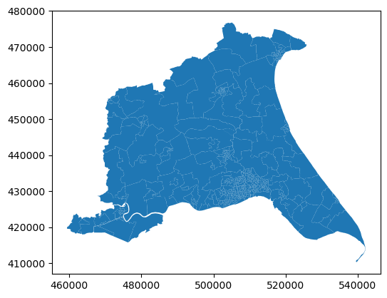
gdf_lsoa_hu = gdf_lsoa_uk[ (gdf_lsoa_uk['LSOA21NM'].str.contains('Kingston upon Hull')) | (gdf_lsoa_uk['LSOA21NM'].str.contains('East Riding of Yorkshire'))]
# transfer the crs
gdf_lsoa_hu = gdf_lsoa_hu.to_crs(epsg=27700)
print(len(gdf_lsoa_hu))
gdf_lsoa_hu.plot()
381
<Axes: >
gdf_lsoa_hu
| FID | LSOA21CD | LSOA21NM | LSOA21NMW | BNG_E | BNG_N | LAT | LONG | Shape__Area | Shape__Length | GlobalID | geometry | |
|---|---|---|---|---|---|---|---|---|---|---|---|---|
| 12115 | 12116 | E01012756 | Kingston upon Hull 025A | 507367 | 430316 | 53.75817 | -0.37294 | 198939.277603 | 3497.174098 | b1f95abf-436c-4f5a-b6e1-93be9e0eb24d | POLYGON ((507433.012 430447.008, 507438.614 43... | |
| 12116 | 12117 | E01012757 | Kingston upon Hull 025B | 508017 | 429519 | 53.75088 | -0.36336 | 318088.364120 | 3716.172876 | 5f00b0d5-45c1-4529-9e08-881c4c58834d | POLYGON ((508039.325 430021.467, 508047.639 42... | |
| 12117 | 12118 | E01012758 | Kingston upon Hull 018A | 507706 | 430320 | 53.75814 | -0.36780 | 311920.300018 | 3772.447527 | 94cd85a6-b982-4038-9625-333de4b818df | POLYGON ((507791.196 430453.312, 507795.719 43... | |
| 12118 | 12119 | E01012759 | Kingston upon Hull 025C | 507184 | 429662 | 53.75233 | -0.37594 | 398184.936035 | 3984.903843 | 1516f69d-ec4e-4e2b-8f3d-81d5f680f631 | POLYGON ((507088.105 429992.978, 507088.215 42... | |
| 12119 | 12120 | E01012760 | Kingston upon Hull 025D | 507714 | 429795 | 53.75342 | -0.36786 | 126002.444229 | 2081.849577 | 2e8144b1-63d2-4100-b2a5-a1fe09759513 | POLYGON ((507913.848 429950.94, 507917.695 429... | |
| ... | ... | ... | ... | ... | ... | ... | ... | ... | ... | ... | ... | ... |
| 33462 | 33463 | E01035468 | Kingston upon Hull 031I | 507220 | 427868 | 53.73621 | -0.37602 | 194811.873474 | 2342.011663 | 41c0a371-996d-4c62-8888-fb4830b71528 | POLYGON ((507209.199 428143.672, 507211.664 42... | |
| 33463 | 33464 | E01035469 | Kingston upon Hull 034C | 509268 | 435508 | 53.80442 | -0.34228 | 602229.054047 | 4797.372241 | ef8cf4ea-28e0-44ba-bdad-f74de2c628c2 | POLYGON ((509524.731 435503.71, 509535.919 435... | |
| 33464 | 33465 | E01035470 | Kingston upon Hull 035A | 508599 | 435590 | 53.80530 | -0.35241 | 512661.485153 | 3739.146033 | f97f0a63-17c4-461a-84e0-f69e41992515 | POLYGON ((508962.524 435417.007, 508963.112 43... | |
| 33465 | 33466 | E01035471 | Kingston upon Hull 035B | 508633 | 435072 | 53.80064 | -0.35207 | 204771.100311 | 2848.973680 | 1dafa6ed-12b8-45cb-a67f-c559fdccfec6 | POLYGON ((508775.831 435260.654, 508776.953 43... | |
| 33466 | 33467 | E01035472 | Kingston upon Hull 035C | 508142 | 434887 | 53.79908 | -0.35959 | 503061.344757 | 3672.250000 | 25c17302-b93b-4752-a042-f2ceadb41dd8 | POLYGON ((507930.326 435252.723, 507986.946 43... |
381 rows × 12 columns
df_crime_hu = pd.read_csv('data/police_humberside_2024/2024-08/2024-08-humberside-street.csv')
df_crime_hu
| Crime ID | Month | Reported by | Falls within | Longitude | Latitude | Location | LSOA code | LSOA name | Crime type | Last outcome category | Context | |
|---|---|---|---|---|---|---|---|---|---|---|---|---|
| 0 | 00c6cf00a107bbc4bfea4bda86cc111d8641d960029de2... | 2024-08 | Humberside Police | Humberside Police | -1.444477 | 53.554880 | On or near Cherrys Road | E01007405 | Barnsley 011D | Violence and sexual offences | Unable to prosecute suspect | NaN |
| 1 | e0b9bd3e5fd219191f6bca6cb730788db2d4a30b49725a... | 2024-08 | Humberside Police | Humberside Police | -1.771430 | 53.719914 | On or near Birkhouse Road | E01010908 | Calderdale 015D | Violence and sexual offences | Status update unavailable | NaN |
| 2 | 5ced08aeab4910f5616a9a491eff404ea79387aad6d863... | 2024-08 | Humberside Police | Humberside Police | -1.570098 | 52.427211 | On or near Mackenzie Close | E01009531 | Coventry 010D | Violence and sexual offences | Action to be taken by another organisation | NaN |
| 3 | 08a2e1a76109963fb73e9583b7954cdbfa7cf8136f6bc6... | 2024-08 | Humberside Police | Humberside Police | -0.956696 | 53.622353 | On or near Maple Road | E01007635 | Doncaster 001D | Violence and sexual offences | Awaiting court outcome | NaN |
| 4 | d76f6945e7b393056c7b1fda351a5d273be1fb7332a87a... | 2024-08 | Humberside Police | Humberside Police | -1.027047 | 53.603907 | On or near Park/Open Space | E01007626 | Doncaster 004B | Violence and sexual offences | Unable to prosecute suspect | NaN |
| ... | ... | ... | ... | ... | ... | ... | ... | ... | ... | ... | ... | ... |
| 8824 | 18c37130d9b4c9d501b20c4ee7b263987d4efd9611d84f... | 2024-08 | Humberside Police | Humberside Police | -1.023274 | 53.711056 | On or near Himsworth Close | E01027885 | Selby 008C | Violence and sexual offences | Status update unavailable | NaN |
| 8825 | 68d04b2c377d180022edfceb558762f546f5948b3d9550... | 2024-08 | Humberside Police | Humberside Police | -1.340161 | 53.342703 | On or near West Street | E01008030 | Sheffield 063A | Violence and sexual offences | Unable to prosecute suspect | NaN |
| 8826 | e24f85c02e60a9b330e0ee8bc2232154749b7629ed8898... | 2024-08 | Humberside Police | Humberside Police | -1.352667 | 54.637803 | On or near Spring Bank Wood | E01033476 | Stockton-on-Tees 005F | Violence and sexual offences | Unable to prosecute suspect | NaN |
| 8827 | 44a158b876156e38830ef93eba54787459556df85a62ef... | 2024-08 | Humberside Police | Humberside Police | -0.222929 | 53.512611 | On or near Grimsby Road | E01026367 | West Lindsey 001A | Violence and sexual offences | Unable to prosecute suspect | NaN |
| 8828 | e0aae955f4c4be84cd9d62300261701efd99117bd71636... | 2024-08 | Humberside Police | Humberside Police | -0.491256 | 53.446820 | On or near Green Lane | E01026411 | West Lindsey 005D | Public order | Unable to prosecute suspect | NaN |
8829 rows × 12 columns
# create the gdf from the df_crime_hu_2024 with x and y coordinates
gdf_crime_hu = gpd.GeoDataFrame(df_crime_hu, geometry=gpd.points_from_xy(df_crime_hu['Longitude'],
                                                                              df_crime_hu['Latitude']), crs='EPSG:4326')
# transform the CRS to EPSG:27700 (British National Grid)
gdf_crime_hu = gdf_crime_hu.to_crs(epsg=27700)
gdf_crime_hu
| Crime ID | Month | Reported by | Falls within | Longitude | Latitude | Location | LSOA code | LSOA name | Crime type | Last outcome category | Context | geometry | |
|---|---|---|---|---|---|---|---|---|---|---|---|---|---|
| 0 | 00c6cf00a107bbc4bfea4bda86cc111d8641d960029de2... | 2024-08 | Humberside Police | Humberside Police | -1.444477 | 53.554880 | On or near Cherrys Road | E01007405 | Barnsley 011D | Violence and sexual offences | Unable to prosecute suspect | NaN | POINT (436900.168 406613.966) |
| 1 | e0b9bd3e5fd219191f6bca6cb730788db2d4a30b49725a... | 2024-08 | Humberside Police | Humberside Police | -1.771430 | 53.719914 | On or near Birkhouse Road | E01010908 | Calderdale 015D | Violence and sexual offences | Status update unavailable | NaN | POINT (415181.204 424856.32) |
| 2 | 5ced08aeab4910f5616a9a491eff404ea79387aad6d863... | 2024-08 | Humberside Police | Humberside Police | -1.570098 | 52.427211 | On or near Mackenzie Close | E01009531 | Coventry 010D | Violence and sexual offences | Action to be taken by another organisation | NaN | POINT (429328.382 281110.253) |
| 3 | 08a2e1a76109963fb73e9583b7954cdbfa7cf8136f6bc6... | 2024-08 | Humberside Police | Humberside Police | -0.956696 | 53.622353 | On or near Maple Road | E01007635 | Doncaster 001D | Violence and sexual offences | Awaiting court outcome | NaN | POINT (469104.345 414482.775) |
| 4 | d76f6945e7b393056c7b1fda351a5d273be1fb7332a87a... | 2024-08 | Humberside Police | Humberside Police | -1.027047 | 53.603907 | On or near Park/Open Space | E01007626 | Doncaster 004B | Violence and sexual offences | Unable to prosecute suspect | NaN | POINT (464479.321 412364.712) |
| ... | ... | ... | ... | ... | ... | ... | ... | ... | ... | ... | ... | ... | ... |
| 8824 | 18c37130d9b4c9d501b20c4ee7b263987d4efd9611d84f... | 2024-08 | Humberside Police | Humberside Police | -1.023274 | 53.711056 | On or near Himsworth Close | E01027885 | Selby 008C | Violence and sexual offences | Status update unavailable | NaN | POINT (464565.252 424288.812) |
| 8825 | 68d04b2c377d180022edfceb558762f546f5948b3d9550... | 2024-08 | Humberside Police | Humberside Police | -1.340161 | 53.342703 | On or near West Street | E01008030 | Sheffield 063A | Violence and sexual offences | Unable to prosecute suspect | NaN | POINT (444029.051 383067.892) |
| 8826 | e24f85c02e60a9b330e0ee8bc2232154749b7629ed8898... | 2024-08 | Humberside Police | Humberside Police | -1.352667 | 54.637803 | On or near Spring Bank Wood | E01033476 | Stockton-on-Tees 005F | Violence and sexual offences | Unable to prosecute suspect | NaN | POINT (441880.904 527155.758) |
| 8827 | 44a158b876156e38830ef93eba54787459556df85a62ef... | 2024-08 | Humberside Police | Humberside Police | -0.222929 | 53.512611 | On or near Grimsby Road | E01026367 | West Lindsey 001A | Violence and sexual offences | Unable to prosecute suspect | NaN | POINT (517938.386 403236.345) |
| 8828 | e0aae955f4c4be84cd9d62300261701efd99117bd71636... | 2024-08 | Humberside Police | Humberside Police | -0.491256 | 53.446820 | On or near Green Lane | E01026411 | West Lindsey 005D | Public order | Unable to prosecute suspect | NaN | POINT (500301.241 395507.5) |
8829 rows × 13 columns
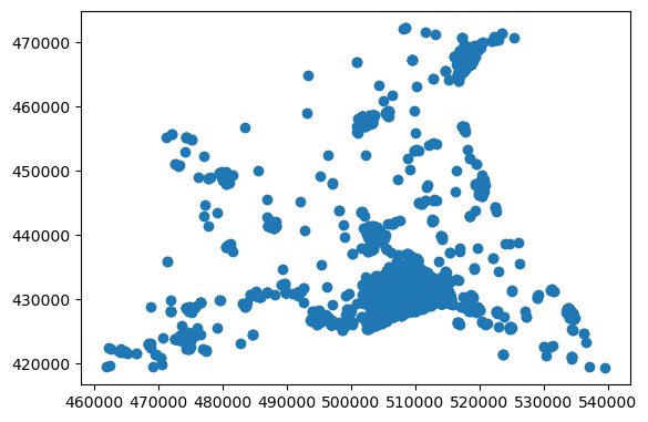
# spatial join the gdf_crime_hu and gdf_lsoa_hull to get the LSOA index for each crime incident (we don't use the 'LSOA codes' in the df_crime_hu_2024)
gdf_crime_hu_lsoa = gpd.sjoin(gdf_crime_hu, gdf_lsoa_hu, how='inner', predicate='within')
gdf_crime_hu_lsoa
| Crime ID | Month | Reported by | Falls within | Longitude | Latitude | Location | LSOA code | LSOA name | Crime type | ... | LSOA21CD | LSOA21NM | LSOA21NMW | BNG_E | BNG_N | LAT | LONG | Shape__Area | Shape__Length | GlobalID | |
|---|---|---|---|---|---|---|---|---|---|---|---|---|---|---|---|---|---|---|---|---|---|
| 16 | NaN | 2024-08 | Humberside Police | Humberside Police | -0.205009 | 54.101015 | On or near Pinfold Grove | E01012934 | East Riding of Yorkshire 001B | Anti-social behaviour | ... | E01012934 | East Riding of Yorkshire 001B | 513910 | 470010 | 54.11338 | -0.25897 | 2.907797e+07 | 27656.377873 | 0ceeaede-a8d0-4686-8d4f-0091b1f243dc | |
| 17 | NaN | 2024-08 | Humberside Police | Humberside Police | -0.208800 | 54.096802 | On or near The Hollows | E01012934 | East Riding of Yorkshire 001B | Anti-social behaviour | ... | E01012934 | East Riding of Yorkshire 001B | 513910 | 470010 | 54.11338 | -0.25897 | 2.907797e+07 | 27656.377873 | 0ceeaede-a8d0-4686-8d4f-0091b1f243dc | |
| 18 | NaN | 2024-08 | Humberside Police | Humberside Police | -0.269446 | 54.124844 | On or near Mere Lane | E01012934 | East Riding of Yorkshire 001B | Anti-social behaviour | ... | E01012934 | East Riding of Yorkshire 001B | 513910 | 470010 | 54.11338 | -0.25897 | 2.907797e+07 | 27656.377873 | 0ceeaede-a8d0-4686-8d4f-0091b1f243dc | |
| 19 | NaN | 2024-08 | Humberside Police | Humberside Police | -0.211149 | 54.096594 | On or near New Pasture Close | E01012934 | East Riding of Yorkshire 001B | Anti-social behaviour | ... | E01012934 | East Riding of Yorkshire 001B | 513910 | 470010 | 54.11338 | -0.25897 | 2.907797e+07 | 27656.377873 | 0ceeaede-a8d0-4686-8d4f-0091b1f243dc | |
| 20 | NaN | 2024-08 | Humberside Police | Humberside Police | -0.210440 | 54.098129 | On or near Ellerburn Drive | E01012934 | East Riding of Yorkshire 001B | Anti-social behaviour | ... | E01012934 | East Riding of Yorkshire 001B | 513910 | 470010 | 54.11338 | -0.25897 | 2.907797e+07 | 27656.377873 | 0ceeaede-a8d0-4686-8d4f-0091b1f243dc | |
| ... | ... | ... | ... | ... | ... | ... | ... | ... | ... | ... | ... | ... | ... | ... | ... | ... | ... | ... | ... | ... | ... |
| 5508 | 4e0999e7dee15e9aaf8a6bfa21bce92b1de5725b1b506e... | 2024-08 | Humberside Police | Humberside Police | -0.348154 | 53.798576 | On or near Halecroft Park | E01033107 | Kingston upon Hull 035E | Other theft | ... | E01033107 | Kingston upon Hull 035E | 508618 | 434547 | 53.79592 | -0.35249 | 3.921917e+05 | 3331.231133 | f698240e-05d9-4a6a-8c12-ba6f537ddef1 | |
| 5509 | 5a22e7a96f1e5df4bb33513cc926d6ac49bc2f34eaea74... | 2024-08 | Humberside Police | Humberside Police | -0.350806 | 53.799107 | On or near Shinewater Park | E01033107 | Kingston upon Hull 035E | Public order | ... | E01033107 | Kingston upon Hull 035E | 508618 | 434547 | 53.79592 | -0.35249 | 3.921917e+05 | 3331.231133 | f698240e-05d9-4a6a-8c12-ba6f537ddef1 | |
| 5510 | 9dab6d637c67dca1f82da99de1bc8853a44a82fd5edd97... | 2024-08 | Humberside Police | Humberside Police | -0.350433 | 53.795452 | On or near Runnymede Way | E01033107 | Kingston upon Hull 035E | Shoplifting | ... | E01033107 | Kingston upon Hull 035E | 508618 | 434547 | 53.79592 | -0.35249 | 3.921917e+05 | 3331.231133 | f698240e-05d9-4a6a-8c12-ba6f537ddef1 | |
| 5511 | 1c068c671bf0613fe0e9264e872d8abfa43e2253bbcb75... | 2024-08 | Humberside Police | Humberside Police | -0.350433 | 53.795452 | On or near Runnymede Way | E01033107 | Kingston upon Hull 035E | Shoplifting | ... | E01033107 | Kingston upon Hull 035E | 508618 | 434547 | 53.79592 | -0.35249 | 3.921917e+05 | 3331.231133 | f698240e-05d9-4a6a-8c12-ba6f537ddef1 | |
| 5512 | cd82f19c01afc3adc33c8567fa1f0a9bdfe4dafccd24b0... | 2024-08 | Humberside Police | Humberside Police | -0.350443 | 53.799453 | On or near Gilderidge Park | E01033107 | Kingston upon Hull 035E | Violence and sexual offences | ... | E01033107 | Kingston upon Hull 035E | 508618 | 434547 | 53.79592 | -0.35249 | 3.921917e+05 | 3331.231133 | f698240e-05d9-4a6a-8c12-ba6f537ddef1 |
5496 rows × 25 columns
gdf_crime_hu_lsoa.plot()
<Axes: >
df_crime_hu_agg = gdf_crime_hu_lsoa.groupby(['LSOA21CD', 'Month']).agg({'Crime ID': 'count'}).reset_index().rename(columns={'Crime ID': 'Numbers'})
df_crime_hu_agg
| LSOA21CD | Month | Numbers | |
|---|---|---|---|
| 0 | E01012756 | 2024-08 | 18 |
| 1 | E01012757 | 2024-08 | 22 |
| 2 | E01012758 | 2024-08 | 16 |
| 3 | E01012759 | 2024-08 | 14 |
| 4 | E01012760 | 2024-08 | 1 |
| ... | ... | ... | ... |
| 372 | E01035467 | 2024-08 | 18 |
| 373 | E01035468 | 2024-08 | 7 |
| 374 | E01035469 | 2024-08 | 11 |
| 375 | E01035470 | 2024-08 | 9 |
| 376 | E01035471 | 2024-08 | 10 |
377 rows × 3 columns
# set the geometry to the df_crime_hull_agg
gdf_crime_hu_agg = pd.merge(gdf_lsoa_hu, df_crime_hu_agg, on='LSOA21CD', how='left')
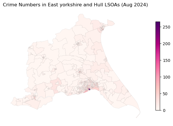
fig, ax = plt.subplots(figsize=(8, 8))
# plot the crime data
gdf_crime_hu_agg.plot(ax=ax, column='Numbers', cmap='RdPu', edgecolor='black', linewidth=0.05, legend=True,
                      legend_kwds={'shrink': 0.5})
ax.set_title('Crime Numbers in East yorkshire and Hull LSOAs (Aug 2024)')
ax.axis('off')
plt.show()
Q2 solution
# read the csv file
df_house_price = pd.read_csv('data/Mean house prices by lower layer super output area- HPSSA dataset 47.csv')
df_house_price_hu = df_house_price[(df_house_price['Local authority name'].str.contains('Hull')) | (df_house_price['Local authority name'].str.contains('East Riding of Yorkshire')) ]
df_house_price_hu
| Local authority code | Local authority name | LSOA code | LSOA name | Year ending Dec 1995 | Year ending Mar 1996 | Year ending Jun 1996 | Year ending Sep 1996 | Year ending Dec 1996 | Year ending Mar 1997 | ... | Year ending Sep 2020 | Year ending Dec 2020 | Year ending Mar 2021 | Year ending Jun 2021 | Year ending Sep 2021 | Year ending Dec 2021 | Year ending Mar 2022 | Year ending Jun 2022 | Year ending Sep 2022 | Year ending Dec 2022 | |
|---|---|---|---|---|---|---|---|---|---|---|---|---|---|---|---|---|---|---|---|---|---|
| 808 | E06000010 | Kingston upon Hull, City of | E01012756 | Kingston upon Hull 025A | 40,920 | 41,652 | 40,819 | 42,748 | 39,059 | 39,567 | ... | 135,647 | 151,126 | 159,225 | 152,954 | 146,913 | 148,260 | 143,033 | 141,745 | 148,008 | 132,769 |
| 809 | E06000010 | Kingston upon Hull, City of | E01012757 | Kingston upon Hull 025B | 31,376 | 29,795 | 30,367 | 30,543 | 30,956 | 32,781 | ... | 132,178 | 123,194 | 127,827 | 135,008 | 141,380 | 148,043 | 135,320 | 139,061 | 130,330 | 137,602 |
| 810 | E06000010 | Kingston upon Hull, City of | E01012758 | Kingston upon Hull 018A | 49,324 | 46,195 | 43,328 | 51,442 | 60,738 | 64,053 | ... | 224,715 | 238,168 | 230,783 | 239,213 | 249,940 | 238,605 | 246,214 | 240,353 | 252,263 | 275,177 |
| 811 | E06000010 | Kingston upon Hull, City of | E01012759 | Kingston upon Hull 025C | 29,197 | 32,087 | 32,336 | 30,748 | 30,246 | 27,783 | ... | 110,625 | 114,500 | 106,262 | 104,782 | 106,537 | 115,615 | 104,722 | 106,965 | 108,325 | 104,977 |
| 812 | E06000010 | Kingston upon Hull, City of | E01012760 | Kingston upon Hull 025D | 28,461 | 28,470 | 27,965 | 28,415 | 28,411 | 28,692 | ... | 94,397 | 93,843 | 92,871 | 95,963 | 98,633 | 102,472 | 108,855 | 114,807 | 121,153 | 124,452 |
| ... | ... | ... | ... | ... | ... | ... | ... | ... | ... | ... | ... | ... | ... | ... | ... | ... | ... | ... | ... | ... | ... |
| 1179 | E06000011 | East Riding of Yorkshire | E01013126 | East Riding of Yorkshire 009E | 70,635 | 64,828 | 60,053 | 66,088 | 72,992 | 78,539 | ... | 324,286 | 332,693 | 336,088 | 345,774 | 349,465 | 378,558 | 389,615 | 411,366 | 463,313 | 455,630 |
| 1180 | E06000011 | East Riding of Yorkshire | E01013127 | East Riding of Yorkshire 018E | 100,765 | 98,318 | 96,342 | 97,912 | 89,962 | 94,182 | ... | 436,643 | 480,611 | 507,417 | 509,694 | 477,282 | 438,554 | 421,262 | 416,400 | 503,722 | 498,563 |
| 1181 | E06000011 | East Riding of Yorkshire | E01032596 | East Riding of Yorkshire 043F | 41,966 | 41,335 | 40,676 | 41,430 | 41,593 | 42,379 | ... | 134,154 | 127,511 | 124,427 | 135,288 | 139,925 | 142,370 | 146,717 | 150,261 | 146,702 | 144,453 |
| 1182 | E06000011 | East Riding of Yorkshire | E01033495 | East Riding of Yorkshire 032G | : | : | : | : | : | : | ... | 152,262 | 204,612 | 214,227 | 227,404 | 222,521 | 209,466 | 203,156 | 183,714 | 194,962 | 195,376 |
| 1183 | E06000011 | East Riding of Yorkshire | E01033496 | East Riding of Yorkshire 032H | 60,974 | 62,406 | 65,388 | 62,199 | 58,120 | 56,913 | ... | 259,775 | 271,633 | 300,098 | 297,239 | 278,697 | 276,424 | 266,227 | 254,792 | 285,688 | 300,487 |
376 rows × 113 columns
gdf_crime_agg_hp = pd.merge(gdf_crime_hu_agg, df_house_price_hu[['LSOA code', 'Year ending Dec 2022']], left_on='LSOA21CD', right_on='LSOA code', how='left')
gdf_crime_agg_hp['Year ending Dec 2022'].values[0]
'132,769'
# we need to do data cleaning for the column 'Year ending Dec 2022'
# the column 'Year ending Dec 2022' is a string, we need to convert it to float
gdf_crime_agg_hp['Year ending Dec 2022'] = gdf_crime_agg_hp['Year ending Dec 2022'].fillna('')
gdf_crime_agg_hp['Year ending Dec 2022'] =  gdf_crime_agg_hp['Year ending Dec 2022'].replace({':': '', ',': ''}, regex=True)
gdf_crime_agg_hp['Year ending Dec 2022'] = gdf_crime_agg_hp['Year ending Dec 2022'].replace('', 0)
gdf_crime_agg_hp['Year ending Dec 2022'] = gdf_crime_agg_hp['Year ending Dec 2022'].astype(float)
gdf_crime_agg_hp = gdf_crime_agg_hp.rename(columns={'Year ending Dec 2022': 'House Price'})
gdf_crime_agg_hp.head()
| FID | LSOA21CD | LSOA21NM | LSOA21NMW | BNG_E | BNG_N | LAT | LONG | Shape__Area | Shape__Length | GlobalID | geometry | Month | Numbers | LSOA code | House Price | |
|---|---|---|---|---|---|---|---|---|---|---|---|---|---|---|---|---|
| 0 | 12116 | E01012756 | Kingston upon Hull 025A | 507367 | 430316 | 53.75817 | -0.37294 | 198939.277603 | 3497.174098 | b1f95abf-436c-4f5a-b6e1-93be9e0eb24d | POLYGON ((507433.012 430447.008, 507438.614 43... | 2024-08 | 18.0 | E01012756 | 132769.0 | |
| 1 | 12117 | E01012757 | Kingston upon Hull 025B | 508017 | 429519 | 53.75088 | -0.36336 | 318088.364120 | 3716.172876 | 5f00b0d5-45c1-4529-9e08-881c4c58834d | POLYGON ((508039.325 430021.467, 508047.639 42... | 2024-08 | 22.0 | E01012757 | 137602.0 | |
| 2 | 12118 | E01012758 | Kingston upon Hull 018A | 507706 | 430320 | 53.75814 | -0.36780 | 311920.300018 | 3772.447527 | 94cd85a6-b982-4038-9625-333de4b818df | POLYGON ((507791.196 430453.312, 507795.719 43... | 2024-08 | 16.0 | E01012758 | 275177.0 | |
| 3 | 12119 | E01012759 | Kingston upon Hull 025C | 507184 | 429662 | 53.75233 | -0.37594 | 398184.936035 | 3984.903843 | 1516f69d-ec4e-4e2b-8f3d-81d5f680f631 | POLYGON ((507088.105 429992.978, 507088.215 42... | 2024-08 | 14.0 | E01012759 | 104977.0 | |
| 4 | 12120 | E01012760 | Kingston upon Hull 025D | 507714 | 429795 | 53.75342 | -0.36786 | 126002.444229 | 2081.849577 | 2e8144b1-63d2-4100-b2a5-a1fe09759513 | POLYGON ((507913.848 429950.94, 507917.695 429... | 2024-08 | 1.0 | E01012760 | 124452.0 |
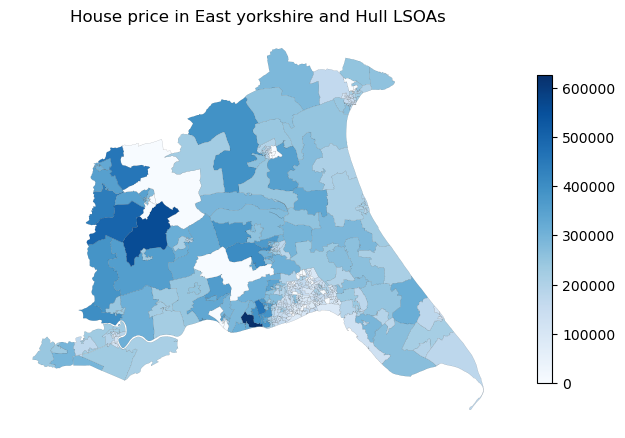
fig, ax = plt.subplots(figsize=(8, 8))
gdf_crime_agg_hp.plot(ax=ax, column='House Price', cmap='Blues', edgecolor='black', linewidth=0.05, legend=True,
                      legend_kwds={'shrink': 0.5})
ax.set_title('House price in East yorkshire and Hull LSOAs')
ax.axis('off')
plt.show()
# read the population data
df_population = pd.read_csv('data/Lower layer Super Output Area population estimates 2019-2022.csv')
df_population.head()
| LAD 2021 Code | LAD 2021 Name | LSOA 2021 Code | LSOA 2021 Name | Total | F0 | F1 | F2 | F3 | F4 | ... | M81 | M82 | M83 | M84 | M85 | M86 | M87 | M88 | M89 | M90 | |
|---|---|---|---|---|---|---|---|---|---|---|---|---|---|---|---|---|---|---|---|---|---|
| 0 | E06000001 | Hartlepool | E01011949 | Hartlepool 009A | 1,870 | 15 | 3 | 11 | 13 | 6 | ... | 6 | 6 | 3 | 3 | 3 | 3 | 2 | 1 | 3 | 1 |
| 1 | E06000001 | Hartlepool | E01011950 | Hartlepool 008A | 1,097 | 6 | 5 | 8 | 8 | 5 | ... | 1 | 1 | 1 | 2 | 0 | 0 | 0 | 0 | 0 | 0 |
| 2 | E06000001 | Hartlepool | E01011951 | Hartlepool 007A | 1,241 | 8 | 7 | 5 | 8 | 3 | ... | 1 | 1 | 3 | 1 | 2 | 2 | 1 | 0 | 1 | 0 |
| 3 | E06000001 | Hartlepool | E01011952 | Hartlepool 002A | 1,615 | 13 | 11 | 17 | 15 | 15 | ... | 0 | 3 | 1 | 2 | 3 | 3 | 4 | 3 | 0 | 13 |
| 4 | E06000001 | Hartlepool | E01011953 | Hartlepool 002B | 1,982 | 9 | 12 | 18 | 11 | 13 | ... | 3 | 4 | 3 | 2 | 0 | 1 | 0 | 0 | 1 | 4 |
5 rows × 187 columns
df_population_hu = df_population[ (df_population['LAD 2021 Name'].str.contains('Kingston upon Hull')) | df_population['LAD 2021 Name'].str.contains('East Riding of Yorkshire')]
df_population_hu.head()
| LAD 2021 Code | LAD 2021 Name | LSOA 2021 Code | LSOA 2021 Name | Total | F0 | F1 | F2 | F3 | F4 | ... | M81 | M82 | M83 | M84 | M85 | M86 | M87 | M88 | M89 | M90 | |
|---|---|---|---|---|---|---|---|---|---|---|---|---|---|---|---|---|---|---|---|---|---|
| 822 | E06000010 | Kingston upon Hull | E01012756 | Kingston upon Hull 025A | 1,477 | 7 | 2 | 4 | 9 | 6 | ... | 5 | 4 | 7 | 5 | 0 | 0 | 0 | 0 | 0 | 0 |
| 823 | E06000010 | Kingston upon Hull | E01012757 | Kingston upon Hull 025B | 1,388 | 4 | 8 | 3 | 6 | 3 | ... | 2 | 1 | 2 | 1 | 2 | 2 | 2 | 4 | 1 | 1 |
| 824 | E06000010 | Kingston upon Hull | E01012758 | Kingston upon Hull 018A | 1,538 | 3 | 5 | 5 | 5 | 4 | ... | 1 | 0 | 2 | 1 | 0 | 2 | 1 | 0 | 0 | 0 |
| 825 | E06000010 | Kingston upon Hull | E01012759 | Kingston upon Hull 025C | 1,670 | 21 | 8 | 18 | 7 | 16 | ... | 1 | 0 | 1 | 3 | 0 | 1 | 1 | 1 | 0 | 2 |
| 826 | E06000010 | Kingston upon Hull | E01012760 | Kingston upon Hull 025D | 1,435 | 10 | 3 | 3 | 10 | 4 | ... | 2 | 1 | 3 | 1 | 0 | 0 | 1 | 0 | 0 | 0 |
5 rows × 187 columns
df_population_hu = df_population_hu[['LSOA 2021 Code', 'Total']]
df_population_hu
| LSOA 2021 Code | Total | |
|---|---|---|
| 822 | E01012756 | 1,477 |
| 823 | E01012757 | 1,388 |
| 824 | E01012758 | 1,538 |
| 825 | E01012759 | 1,670 |
| 826 | E01012760 | 1,435 |
| ... | ... | ... |
| 1198 | E01034756 | 2,488 |
| 1199 | E01034757 | 1,209 |
| 1200 | E01034758 | 1,758 |
| 1201 | E01034759 | 1,681 |
| 1202 | E01034760 | 1,469 |
381 rows × 2 columns
# merge the population data with the gdf_crime_hull_agg_hp
gdf_crime_agg_hp_pop = pd.merge(gdf_crime_agg_hp, df_population_hu, left_on='LSOA21CD', right_on='LSOA 2021 Code', how='left')
gdf_crime_agg_hp_pop.head()
| FID | LSOA21CD | LSOA21NM | LSOA21NMW | BNG_E | BNG_N | LAT | LONG | Shape__Area | Shape__Length | GlobalID | geometry | Month | Numbers | LSOA code | House Price | LSOA 2021 Code | Total | |
|---|---|---|---|---|---|---|---|---|---|---|---|---|---|---|---|---|---|---|
| 0 | 12116 | E01012756 | Kingston upon Hull 025A | 507367 | 430316 | 53.75817 | -0.37294 | 198939.277603 | 3497.174098 | b1f95abf-436c-4f5a-b6e1-93be9e0eb24d | POLYGON ((507433.012 430447.008, 507438.614 43... | 2024-08 | 18.0 | E01012756 | 132769.0 | E01012756 | 1,477 | |
| 1 | 12117 | E01012757 | Kingston upon Hull 025B | 508017 | 429519 | 53.75088 | -0.36336 | 318088.364120 | 3716.172876 | 5f00b0d5-45c1-4529-9e08-881c4c58834d | POLYGON ((508039.325 430021.467, 508047.639 42... | 2024-08 | 22.0 | E01012757 | 137602.0 | E01012757 | 1,388 | |
| 2 | 12118 | E01012758 | Kingston upon Hull 018A | 507706 | 430320 | 53.75814 | -0.36780 | 311920.300018 | 3772.447527 | 94cd85a6-b982-4038-9625-333de4b818df | POLYGON ((507791.196 430453.312, 507795.719 43... | 2024-08 | 16.0 | E01012758 | 275177.0 | E01012758 | 1,538 | |
| 3 | 12119 | E01012759 | Kingston upon Hull 025C | 507184 | 429662 | 53.75233 | -0.37594 | 398184.936035 | 3984.903843 | 1516f69d-ec4e-4e2b-8f3d-81d5f680f631 | POLYGON ((507088.105 429992.978, 507088.215 42... | 2024-08 | 14.0 | E01012759 | 104977.0 | E01012759 | 1,670 | |
| 4 | 12120 | E01012760 | Kingston upon Hull 025D | 507714 | 429795 | 53.75342 | -0.36786 | 126002.444229 | 2081.849577 | 2e8144b1-63d2-4100-b2a5-a1fe09759513 | POLYGON ((507913.848 429950.94, 507917.695 429... | 2024-08 | 1.0 | E01012760 | 124452.0 | E01012760 | 1,435 |
gdf_crime_agg_hp_pop.Total.values
array(['1,477', '1,388', '1,538', '1,670', '1,435', '1,769', '1,339',
       '1,706', '1,179', '1,391', '1,376', '1,559', '1,314', '1,325',
       '1,594', '1,580', '1,545', '1,534', '1,497', '1,627', '1,403',
       '1,557', '1,381', '1,328', '1,800', '1,280', '1,451', '1,294',
       '2,009', '1,323', '1,260', '1,456', '1,437', '1,290', '1,340',
       '1,633', '1,526', '1,428', '1,404', '1,993', '1,204', '1,312',
       '1,671', '1,225', '1,381', '1,430', '1,342', '1,368', '1,660',
       '1,365', '1,448', '1,378', '1,698', '1,758', '1,837', '1,547',
       '1,320', '1,611', '1,487', '1,508', '1,461', '1,424', '1,214',
       '1,377', '1,316', '1,913', '1,585', '2,005', '1,452', '1,614',
       '1,472', '1,791', '1,391', '1,836', '1,597', '1,739', '1,041',
       '1,445', '1,605', '1,672', '1,338', '1,555', '1,582', '1,435',
       '1,691', '1,286', '1,505', '1,346', '1,264', '1,707', '1,532',
       '1,714', '1,675', '2,175', '2,145', '1,726', '1,825', '2,256',
       '1,650', '2,404', '1,383', '2,441', '1,766', '1,311', '1,754',
       '1,745', '1,876', '1,649', '1,807', '1,673', '1,599', '1,491',
       '1,515', '1,703', '1,670', '1,570', '1,851', '1,410', '1,776',
       '1,509', '1,545', '1,462', '1,899', '1,581', '1,529', '1,607',
       '1,645', '2,420', '2,034', '1,659', '2,193', '1,903', '1,673',
       '1,465', '1,590', '1,448', '1,527', '1,644', '1,215', '1,320',
       '1,576', '1,448', '1,037', '1,176', '1,205', '1,136', '1,629',
       '1,993', '3,612', '1,553', '1,905', '1,900', '1,695', '1,437',
       '1,165', '1,496', '2,176', '1,671', '1,345', '2,324', '1,474',
       '1,701', '1,869', '1,372', '1,526', '1,679', '1,015', '1,818',
       '1,340', '1,166', '2,101', '1,896', '1,544', '1,303', '1,212',
       '1,703', '1,402', '1,491', '1,565', '1,378', '1,394', '1,341',
       '1,317', '1,190', '1,512', '1,379', '1,624', '1,619', '1,192',
       '1,380', '1,039', '1,449', '1,628', '2,301', '1,266', '1,497',
       '1,730', '1,245', '1,597', '1,631', '1,096', '1,810', '1,583',
       '1,544', '1,628', '1,358', '1,753', '1,710', '1,680', '1,325',
       '1,537', '1,784', '1,910', '1,722', '1,540', '1,698', '1,577',
       '1,830', '1,411', '1,589', '1,407', '1,421', '1,846', '1,958',
       '1,711', '1,905', '2,246', '1,732', '2,210', '1,891', '1,760',
       '1,521', '1,837', '2,150', '1,488', '1,491', '1,366', '1,599',
       '1,419', '1,597', '1,808', '1,409', '1,367', '1,747', '1,811',
       '2,101', '1,954', '1,869', '1,896', '1,431', '1,982', '1,868',
       '1,917', '1,308', '1,663', '1,758', '1,540', '1,460', '1,364',
       '1,401', '1,434', '1,562', '1,800', '1,463', '1,447', '1,382',
       '1,471', '2,208', '2,351', '1,581', '1,549', '1,362', '1,995',
       '1,533', '1,582', '1,561', '2,328', '1,652', '1,742', '1,698',
       '1,915', '1,889', '1,898', '1,590', '1,672', '1,489', '1,652',
       '2,448', '1,568', '1,626', '1,442', '1,337', '1,593', '1,539',
       '1,610', '2,321', '1,578', '1,454', '1,558', '1,767', '1,827',
       '1,589', '1,377', '1,518', '2,097', '1,440', '1,540', '1,395',
       '1,503', '1,648', '1,394', '1,295', '1,737', '1,405', '1,357',
       '2,029', '1,707', '1,420', '1,518', '2,662', '1,613', '1,387',
       '1,509', '1,778', '1,273', '2,217', '1,406', '1,631', '1,596',
       '1,408', '1,371', '1,096', '1,417', '1,171', '2,171', '1,762',
       '1,531', '1,366', '1,438', '1,524', '1,536', '1,421', '1,854',
       '1,459', '1,463', '1,475', '2,052', '2,311', '1,488', '2,153',
       '2,231', '1,635', '2,283', '1,635', '1,857', '1,398', '1,533',
       '1,511', '1,313', '1,430', '1,475', '1,587', '1,488', '1,164',
       '1,239', '1,800', '2,488', '1,209', '1,758', '1,681', '1,469',
       '2,397', '2,326', '1,240', '1,342', '1,782', '1,192', '2,406',
       '2,819', '1,291', '1,768'], dtype=object)
# we need to rename the column 'Total' to 'Population' and do data cleaning
gdf_crime_agg_hp_pop['Total'] = gdf_crime_agg_hp_pop['Total'].replace({ ',': ''}, regex=True).astype(float)
gdf_crime_agg_hp_pop = gdf_crime_agg_hp_pop.rename(columns={'Total': 'Population'})
gdf_crime_agg_hp_pop
| FID | LSOA21CD | LSOA21NM | LSOA21NMW | BNG_E | BNG_N | LAT | LONG | Shape__Area | Shape__Length | GlobalID | geometry | Month | Numbers | LSOA code | House Price | LSOA 2021 Code | Population | |
|---|---|---|---|---|---|---|---|---|---|---|---|---|---|---|---|---|---|---|
| 0 | 12116 | E01012756 | Kingston upon Hull 025A | 507367 | 430316 | 53.75817 | -0.37294 | 198939.277603 | 3497.174098 | b1f95abf-436c-4f5a-b6e1-93be9e0eb24d | POLYGON ((507433.012 430447.008, 507438.614 43... | 2024-08 | 18.0 | E01012756 | 132769.0 | E01012756 | 1477.0 | |
| 1 | 12117 | E01012757 | Kingston upon Hull 025B | 508017 | 429519 | 53.75088 | -0.36336 | 318088.364120 | 3716.172876 | 5f00b0d5-45c1-4529-9e08-881c4c58834d | POLYGON ((508039.325 430021.467, 508047.639 42... | 2024-08 | 22.0 | E01012757 | 137602.0 | E01012757 | 1388.0 | |
| 2 | 12118 | E01012758 | Kingston upon Hull 018A | 507706 | 430320 | 53.75814 | -0.36780 | 311920.300018 | 3772.447527 | 94cd85a6-b982-4038-9625-333de4b818df | POLYGON ((507791.196 430453.312, 507795.719 43... | 2024-08 | 16.0 | E01012758 | 275177.0 | E01012758 | 1538.0 | |
| 3 | 12119 | E01012759 | Kingston upon Hull 025C | 507184 | 429662 | 53.75233 | -0.37594 | 398184.936035 | 3984.903843 | 1516f69d-ec4e-4e2b-8f3d-81d5f680f631 | POLYGON ((507088.105 429992.978, 507088.215 42... | 2024-08 | 14.0 | E01012759 | 104977.0 | E01012759 | 1670.0 | |
| 4 | 12120 | E01012760 | Kingston upon Hull 025D | 507714 | 429795 | 53.75342 | -0.36786 | 126002.444229 | 2081.849577 | 2e8144b1-63d2-4100-b2a5-a1fe09759513 | POLYGON ((507913.848 429950.94, 507917.695 429... | 2024-08 | 1.0 | E01012760 | 124452.0 | E01012760 | 1435.0 | |
| ... | ... | ... | ... | ... | ... | ... | ... | ... | ... | ... | ... | ... | ... | ... | ... | ... | ... | ... |
| 376 | 33463 | E01035468 | Kingston upon Hull 031I | 507220 | 427868 | 53.73621 | -0.37602 | 194811.873474 | 2342.011663 | 41c0a371-996d-4c62-8888-fb4830b71528 | POLYGON ((507209.199 428143.672, 507211.664 42... | 2024-08 | 7.0 | NaN | 0.0 | E01035468 | 1192.0 | |
| 377 | 33464 | E01035469 | Kingston upon Hull 034C | 509268 | 435508 | 53.80442 | -0.34228 | 602229.054047 | 4797.372241 | ef8cf4ea-28e0-44ba-bdad-f74de2c628c2 | POLYGON ((509524.731 435503.71, 509535.919 435... | 2024-08 | 11.0 | NaN | 0.0 | E01035469 | 2406.0 | |
| 378 | 33465 | E01035470 | Kingston upon Hull 035A | 508599 | 435590 | 53.80530 | -0.35241 | 512661.485153 | 3739.146033 | f97f0a63-17c4-461a-84e0-f69e41992515 | POLYGON ((508962.524 435417.007, 508963.112 43... | 2024-08 | 9.0 | NaN | 0.0 | E01035470 | 2819.0 | |
| 379 | 33466 | E01035471 | Kingston upon Hull 035B | 508633 | 435072 | 53.80064 | -0.35207 | 204771.100311 | 2848.973680 | 1dafa6ed-12b8-45cb-a67f-c559fdccfec6 | POLYGON ((508775.831 435260.654, 508776.953 43... | 2024-08 | 10.0 | NaN | 0.0 | E01035471 | 1291.0 | |
| 380 | 33467 | E01035472 | Kingston upon Hull 035C | 508142 | 434887 | 53.79908 | -0.35959 | 503061.344757 | 3672.250000 | 25c17302-b93b-4752-a042-f2ceadb41dd8 | POLYGON ((507930.326 435252.723, 507986.946 43... | NaN | NaN | NaN | 0.0 | E01035472 | 1768.0 |
381 rows × 18 columns
gdf_crime_agg_hp_pop['Numbers'] = gdf_crime_agg_hp_pop['Numbers'].fillna(0)
gdf_crime_agg_hp_pop['House Price'] = gdf_crime_agg_hp_pop['House Price'].fillna(0)
gdf_crime_agg_hp_pop['Population'] = gdf_crime_agg_hp_pop['Population'].fillna(0)
Q3 solution
import libpysal.weights as weights
# use the SlM, SEM and SDM to do the spatial regression
# set the y and X variables
y = gdf_crime_agg_hp_pop[['Numbers']].values
X = gdf_crime_agg_hp_pop[['House Price', 'Population']].values
# set the spatial weights
w_lsoa  = weights.Queen.from_dataframe(gdf_crime_agg_hp_pop, use_index='True')
w = w_lsoa
w.transform = 'R'  # Row-standardized

# Fit spatial lag model
model_sl = ML_Lag(y, X, w=w, name_y='Numbers', name_x=['House Price', 'Population'], name_w='Queen', name_ds='East yorkshire and Hull')
# Output summary
print(model_sl.summary)
REGRESSION RESULTS
------------------

SUMMARY OF OUTPUT: MAXIMUM LIKELIHOOD SPATIAL LAG (METHOD = FULL)
-----------------------------------------------------------------
Data set            :East yorkshire and Hull
Weights matrix      :       Queen
Dependent Variable  :     Numbers                Number of Observations:         381
Mean dependent var  :     13.1417                Number of Variables   :           4
S.D. dependent var  :     17.8143                Degrees of Freedom    :         377
Pseudo R-squared    :      0.2035
Spatial Pseudo R-squared:  0.1112
Log likelihood      :  -1601.4457
Sigma-square ML     :    253.8232                Akaike info criterion :    3210.891
S.E of regression   :     15.9318                Schwarz criterion     :    3226.663

------------------------------------------------------------------------------------
            Variable     Coefficient       Std.Error     z-Statistic     Probability
------------------------------------------------------------------------------------
            CONSTANT         7.88095         4.64113         1.69807         0.08950
         House Price        -0.00003         0.00001        -3.93716         0.00008
          Population         0.00368         0.00262         1.40820         0.15907
           W_Numbers         0.39369         0.06406         6.14562         0.00000
------------------------------------------------------------------------------------

SPATIAL LAG MODEL IMPACTS
Impacts computed using the 'simple' method.
            Variable         Direct        Indirect          Total
         House Price        -0.0000         -0.0000         -0.0001
          Population         0.0037          0.0024          0.0061
================================ END OF REPORT =====================================
# Fit spatial error model
model_sem = ML_Error(y, X, w=w, name_y='Numbers', name_x=['House Price', 'Population'], name_w='Queen', name_ds='East yorkshire and Hull')
# Output summary
print(model_sem.summary)
REGRESSION RESULTS
------------------

SUMMARY OF OUTPUT: ML SPATIAL ERROR (METHOD = full)
---------------------------------------------------
Data set            :East yorkshire and Hull
Weights matrix      :       Queen
Dependent Variable  :     Numbers                Number of Observations:         381
Mean dependent var  :     13.1417                Number of Variables   :           3
S.D. dependent var  :     17.8143                Degrees of Freedom    :         378
Pseudo R-squared    :      0.0858
Log likelihood      :  -1604.2593
Sigma-square ML     :    257.5623                Akaike info criterion :    3214.519
S.E of regression   :     16.0487                Schwarz criterion     :    3226.347

------------------------------------------------------------------------------------
            Variable     Coefficient       Std.Error     z-Statistic     Probability
------------------------------------------------------------------------------------
            CONSTANT        12.51763         4.97003         2.51862         0.01178
         House Price        -0.00003         0.00001        -3.14638         0.00165
          Population         0.00375         0.00274         1.36661         0.17175
              lambda         0.39451         0.06546         6.02678         0.00000
------------------------------------------------------------------------------------
================================ END OF REPORT =====================================
# Fit spatial lag model
model_dur = ML_Lag(y, X, w=w, name_y='Numbers', name_x=['House Price', 'Population'], name_w='Queen', name_ds='East yorkshire and Hull')

# Output summary
print(model_dur.summary)
REGRESSION RESULTS
------------------

SUMMARY OF OUTPUT: MAXIMUM LIKELIHOOD SPATIAL LAG (METHOD = FULL)
-----------------------------------------------------------------
Data set            :East yorkshire and Hull
Weights matrix      :       Queen
Dependent Variable  :     Numbers                Number of Observations:         381
Mean dependent var  :     13.1417                Number of Variables   :           4
S.D. dependent var  :     17.8143                Degrees of Freedom    :         377
Pseudo R-squared    :      0.2035
Spatial Pseudo R-squared:  0.1112
Log likelihood      :  -1601.4457
Sigma-square ML     :    253.8232                Akaike info criterion :    3210.891
S.E of regression   :     15.9318                Schwarz criterion     :    3226.663

------------------------------------------------------------------------------------
            Variable     Coefficient       Std.Error     z-Statistic     Probability
------------------------------------------------------------------------------------
            CONSTANT         7.88095         4.64113         1.69807         0.08950
         House Price        -0.00003         0.00001        -3.93716         0.00008
          Population         0.00368         0.00262         1.40820         0.15907
           W_Numbers         0.39369         0.06406         6.14562         0.00000
------------------------------------------------------------------------------------

SPATIAL LAG MODEL IMPACTS
Impacts computed using the 'simple' method.
            Variable         Direct        Indirect          Total
         House Price        -0.0000         -0.0000         -0.0001
          Population         0.0037          0.0024          0.0061
================================ END OF REPORT =====================================