Week7 Lab Tutorial Timeline

Time	Activity
16:00–16:05	Introduction — Overview of the main tasks for the lab tutorials
16:05–16:45	Tutorial: Clustering for spatial and temporal big data — Follow Section 7.1 of the Jupyter Notebook to practice the GMM, KMeans and DBSCAN
16:45–17:30	Tutorial: Clustering for spatial and temporal big data — Follow Section 7.2-7.3 of the Jupyter Notebook to practice the DB index, Silhouette coefficient and ST-DBSCAN
17:30–17:55	Quiz — Complete quiz tasks
17:55–18:00	Wrap-up — Recap key points and address final questions

For this module’s lab tutorials, you can download all the required data using the provided link (click).

Please make sure that both the Jupyter Notebook file and the data and img folder are placed in the same directory (specifically within the STBDA_lab folder) to ensure the code runs correctly.

Week 7 Key Takeaways:

• Understand the concept of clustering and its applications in spatial and temporal big data.

• Learn how to apply clustering algorithms such as Gaussian Mixture Model (GMM), KMeans, and DBSCAN to spatial data.

• Explore the use of clustering in road accident data analysis.

• Gain insights into parameter tuning in clustering, including the use of Silhouette Coefficient and Davies-Bouldin Index.

• Understand the concept of spatial and temporal clustering and its applications in human mobility analysis.

• Learn how to apply ST-DBSCAN for clustering spatio-temporal data.

7 Clustering for spatial and temporal big data

Clustering is a machine learning method (unsupervised learning) that groups a collection of objects into clusters, with each cluster containing objects that are highly similar to each other and distinct from those in other clusters.

7.1 Spatial Clustering

Spatial clustering is a method used in spatial data analysis to group together objects or data points mainly based on their spatial (geographical) location. The goal is to identify regions/areas where the data points/objects are more similar to each other than to those in other regions/areas.

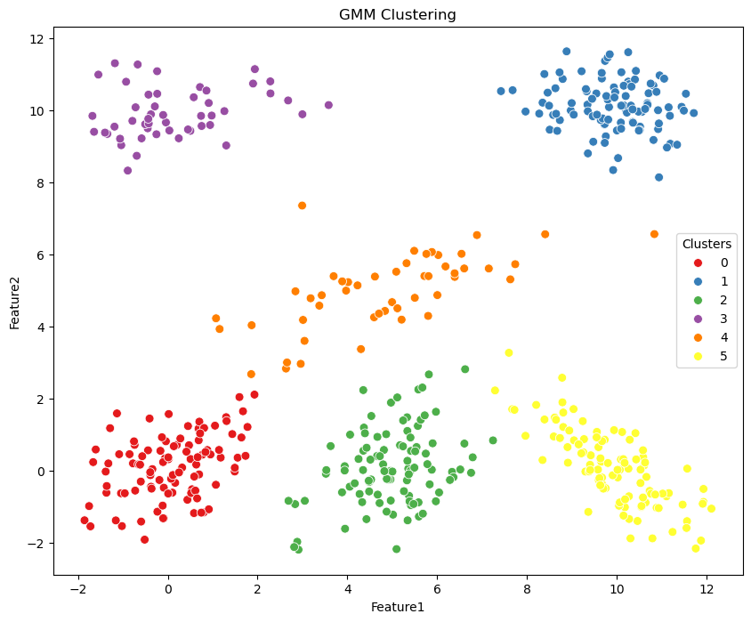
7.1.1 Gaussian Mixture Model (GMM)

A Gaussian Mixture Model (GMM) is a probabilistic model that assumes that the data is generated from a mixture of several Gaussian distributions with unknown parameters. The equation for a GMM is a weighted sum of multiple Gaussian (Normal) distributions. The model is defined as:

\(p(x) = \sum_{i=1}^{K} w_i \mathcal{N}({x}|\mu_i, \sigma_i)\)

• \( p(x)\) overall probability

• \( {x} \) is the data point.

• \( K \) is the total number of Gaussian (a normal distribution as a cluster).

• \( w_i \) are the weights (size) of the \(i\)th Gaussian (summing to 1).

• \( \mathcal{N}({x}|\mu_i, \sigma_i) \) is the probability of the \(i\)th Gaussian.

• \(\mu_i\) is the mean of the \(i\)th Gaussian.

• \(\sigma_i\) is the variance of the \(i\)th Gaussian.

import pandas as pd
import matplotlib.pyplot as plt
import numpy as np
import warnings
warnings.filterwarnings('ignore')

# Read the data
df = pd.read_csv('data/cluster_data.csv')

df

	Feature1	Feature2
0	4.862775	1.011907
1	5.743938	0.472795
2	10.177229	-1.014992
3	-0.405046	1.447232
4	1.260348	9.982292
...	...	...
495	9.447088	10.323605
496	5.335410	0.273029
497	5.668767	2.307601
498	8.489488	10.133309
499	6.282093	-0.258828

500 rows × 2 columns

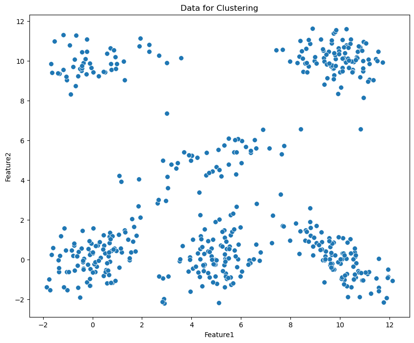
# Plot the data using seaborn
import seaborn as sns
plt.figure(figsize=(10, 8))
g = sns.scatterplot(data=df, x='Feature1', y='Feature2', s=50)
g.set_title('Data for Clustering')
plt.show()

from sklearn.mixture import GaussianMixture

from sklearn.mixture import GaussianMixture
# Define the parameters for GMM
gmm = GaussianMixture(n_components=6, covariance_type='full', random_state=50) 
# GMM fitting
gmm.fit(df[['Feature1', 'Feature2']]) 
# Get labels from clusters
gmm_labels = gmm.predict(df[['Feature1', 'Feature2']])

# Assign the labels of clusters to df
df['gmm_labels']=gmm_labels

# Plot the data with clusters
plt.figure(figsize=(10, 8))
g = sns.scatterplot(data=df, x='Feature1', y='Feature2', hue='gmm_labels', palette='Set1', s=50, legend=True)
g.set_title('GMM Clustering')
g.legend(title='Clusters', loc='center right')
plt.show()

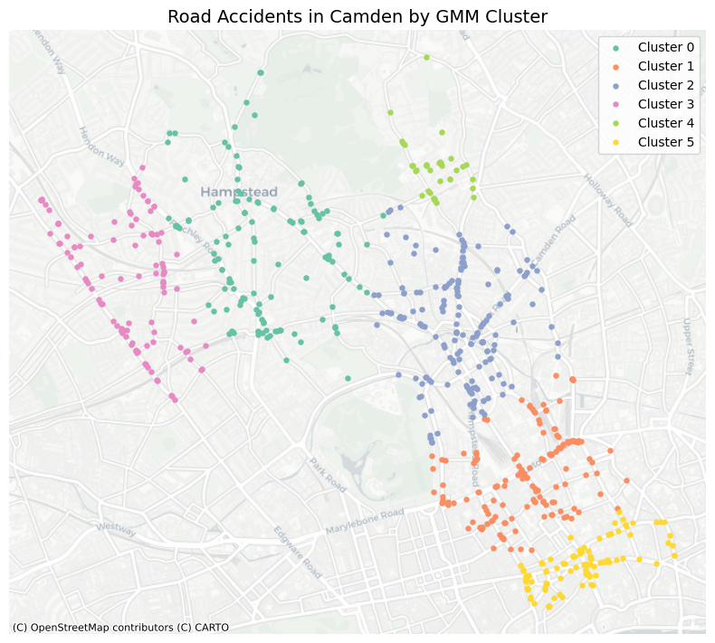
Applying GMM clustering on road accidents

In this section, we will apply GMM to the road accident data in Camden Town, London, to identify clusters of accidents based on their spatial distribution. The dataset contains information about road accidents, including their geographical coordinates. You can find the dataset here.

In spatial analysis, use projected coordinates, such as the UK National Grid, instead of GPS coordinates (latitude and longitude) in clustering.

• Projected Coordinates: In a projected coordinate system (e.g., the UK National Grid), distances are measured in consistent units (e.g., meters). This makes the process straightforward to compute distances and areas accurately and make the results understandable.

• GPS Coordinates: Latitude and longitude are in degrees, and the actual distance represented by one degree varies depending on the location on the Earth’s surface. The Earth’s curvature affects calculations, requiring more complex spherical trigonometry for accurate distance and area computations.

# Read the road accident data
df_accident = pd.read_csv('data/dft-road-casualty-statistics-collision-2023.csv')

df_accident

	accident_index	accident_year	accident_reference	location_easting_osgr	location_northing_osgr	longitude	latitude	police_force	accident_severity	number_of_vehicles	...	light_conditions	weather_conditions	road_surface_conditions	special_conditions_at_site	carriageway_hazards	urban_or_rural_area	did_police_officer_attend_scene_of_accident	trunk_road_flag	lsoa_of_accident_location	enhanced_severity_collision
0	2023010419171	2023	10419171	525060.0	170416.0	-0.202878	51.418974	1	3	1	...	4	8	2	0	0	1	1	2	E01003383	-1
1	2023010419183	2023	10419183	535463.0	198745.0	-0.042464	51.671155	1	3	3	...	4	1	1	0	0	1	1	2	E01001547	-1
2	2023010419189	2023	10419189	508702.0	177696.0	-0.435789	51.487777	1	3	2	...	4	1	1	0	0	1	1	2	E01002448	-1
3	2023010419191	2023	10419191	520341.0	190175.0	-0.263972	51.597575	1	3	2	...	4	9	1	0	0	1	1	2	E01000129	-1
4	2023010419192	2023	10419192	527255.0	176963.0	-0.168976	51.477324	1	3	2	...	4	1	1	0	0	1	1	2	E01004583	-1
...	...	...	...	...	...	...	...	...	...	...	...	...	...	...	...	...	...	...	...	...	...
104253	2023991452286	2023	991452286	246754.0	661133.0	-4.447490	55.819059	99	2	1	...	5	2	2	-1	-1	1	1	-1	-1	7
104254	2023991452640	2023	991452640	224491.0	581627.0	-4.752200	55.097920	99	3	2	...	1	9	1	0	0	2	2	-1	-1	3
104255	2023991453360	2023	991453360	383341.0	806427.0	-2.276957	57.148422	99	3	2	...	4	2	2	-1	-1	1	1	-1	-1	3
104256	2023991461915	2023	991461915	271662.0	655488.0	-4.047591	55.775637	99	3	1	...	4	8	1	-1	-1	1	1	-1	-1	3
104257	2023991462793	2023	991462793	327349.0	666746.0	-3.163102	55.888350	99	3	2	...	1	1	1	0	0	2	1	-1	-1	3

104258 rows × 37 columns

df_accident.columns

Index(['accident_index', 'accident_year', 'accident_reference',
       'location_easting_osgr', 'location_northing_osgr', 'longitude',
       'latitude', 'police_force', 'accident_severity', 'number_of_vehicles',
       'number_of_casualties', 'date', 'day_of_week', 'time',
       'local_authority_district', 'local_authority_ons_district',
       'local_authority_highway', 'first_road_class', 'first_road_number',
       'road_type', 'speed_limit', 'junction_detail', 'junction_control',
       'second_road_class', 'second_road_number',
       'pedestrian_crossing_human_control',
       'pedestrian_crossing_physical_facilities', 'light_conditions',
       'weather_conditions', 'road_surface_conditions',
       'special_conditions_at_site', 'carriageway_hazards',
       'urban_or_rural_area', 'did_police_officer_attend_scene_of_accident',
       'trunk_road_flag', 'lsoa_of_accident_location',
       'enhanced_severity_collision'],
      dtype='object')

# Camden Town LSOA index
camden_lsoas = ['E01000936', 'E01000937', 'E01000964', 'E01000934', 'E01000935', 'E01000942', 'E01000932', 'E01000933',
                'E01000930', 'E01000931', 'E01000938', 'E01000939', 'E01000943', 'E01000916', 'E01000917', 'E01000914',
                'E01000915', 'E01000912', 'E01000913', 'E01000910', 'E01000911', 'E01000918', 'E01000919', 'E01000876',
                'E01000877', 'E01000874', 'E01000875', 'E01000872', 'E01000873', 'E01000870', 'E01000871', 'E01000878',
                'E01000879', 'E01000966', 'E01000940', 'E01000967', 'E01000965', 'E01000962', 'E01000963', 'E01000960',
                'E01000961', 'E01000941', 'E01000968', 'E01000949', 'E01000969', 'E01000856', 'E01000857', 'E01000854',
                'E01000855', 'E01000852', 'E01000853', 'E01000850', 'E01000851', 'E01000858', 'E01000859', 'E01000946',
                'E01000947', 'E01000944', 'E01000890', 'E01000899', 'E01000945', 'E01000948', 'E01000926', 'E01000927',
                'E01000924', 'E01000925', 'E01000922', 'E01000905', 'E01000923', 'E01000955', 'E01000920', 'E01000921',
                'E01000928', 'E01000929', 'E01000950', 'E01000897', 'E01000896', 'E01000895', 'E01000894', 'E01000893',
                'E01000892', 'E01000891', 'E01000898', 'E01000906', 'E01000907', 'E01000904', 'E01000902', 'E01000903',
                'E01000900', 'E01000901', 'E01000908', 'E01000909', 'E01000866', 'E01000867', 'E01000951', 'E01000864',
                'E01000865', 'E01000862', 'E01000863', 'E01000860', 'E01000861', 'E01000868', 'E01000869', 'E01000846',
                'E01000847', 'E01000844', 'E01000845', 'E01000842', 'E01000843', 'E01000848', 'E01000849', 'E01000974',
                'E01000972', 'E01000973', 'E01000970', 'E01000971', 'E01000956', 'E01000957', 'E01000954', 'E01000952',
                'E01000953', 'E01000958', 'E01000959', 'E01000887', 'E01000886', 'E01000885', 'E01000884', 'E01000883',
                'E01000882', 'E01000881', 'E01000880', 'E01000889', 'E01000888']
print('The number of LSOAs in Camden Town:', len(camden_lsoas))

The number of LSOAs in Camden Town: 133

df_accident_camden = df_accident.query('lsoa_of_accident_location in @camden_lsoas')

df_accident_camden

	accident_index	accident_year	accident_reference	location_easting_osgr	location_northing_osgr	longitude	latitude	police_force	accident_severity	number_of_vehicles	...	light_conditions	weather_conditions	road_surface_conditions	special_conditions_at_site	carriageway_hazards	urban_or_rural_area	did_police_officer_attend_scene_of_accident	trunk_road_flag	lsoa_of_accident_location	enhanced_severity_collision
5	2023010419198	2023	10419198	524780.0	184471.0	-0.201941	51.545349	1	3	1	...	4	1	1	0	0	1	1	2	E01000974	-1
20	2023010419281	2023	10419281	525522.0	184858.0	-0.191108	51.548662	1	2	1	...	4	2	2	0	0	1	1	2	E01000973	-1
21	2023010419282	2023	10419282	530049.0	184288.0	-0.126067	51.542516	1	3	1	...	4	2	2	0	0	1	1	2	E01000868	-1
48	2023010419391	2023	10419391	528183.0	184396.0	-0.152921	51.543913	1	2	2	...	4	1	1	0	0	1	1	2	E01000906	-1
52	2023010419398	2023	10419398	526452.0	185517.0	-0.177466	51.554377	1	3	2	...	4	1	1	0	0	1	3	2	E01000879	-1
...	...	...	...	...	...	...	...	...	...	...	...	...	...	...	...	...	...	...	...	...	...
22654	2023010487700	2023	10487700	529836.0	181379.0	-0.130208	51.516423	1	2	1	...	4	1	1	0	9	1	3	2	E01000855	-1
22687	2023010491078	2023	10491078	529537.0	181828.0	-0.134350	51.520526	1	3	2	...	1	1	1	9	0	1	3	2	E01000851	-1
22695	2023010494344	2023	10494344	526857.0	184926.0	-0.171841	51.548975	1	2	2	...	1	1	1	0	0	1	1	2	E01000882	-1
22731	2023011366792	2023	11366792	530953.0	181613.0	-0.114033	51.518268	1	3	2	...	1	1	1	0	0	1	1	2	E01000914	3
87863	2023481407567	2023	481407567	531350.0	181567.0	-0.108331	51.517763	48	2	1	...	4	8	2	0	0	1	3	2	E01000917	5

722 rows × 37 columns

# we notice only 125/133 LSOAs have road accidents in Camden Town, 2023
df_accident_camden.lsoa_of_accident_location.nunique()

125

# plot the data using folium
import folium
# Create a map centered around Camden Town
m = folium.Map(location=[51.5416, -0.1425], zoom_start=13)
# we use the basemap layer from cartoons
folium.TileLayer('cartodb positron').add_to(m)
# Add road accidents to the map
for _, row in df_accident_camden.iterrows():
    folium.CircleMarker(
        location=[row['latitude'], row['longitude']],
        radius=3,
        color='Royalblue',
        fill=True,
        fill_color='Royalblue',
        fill_opacity=0.8
    ).add_to(m)
m

Make this Notebook Trusted to load map: File -> Trust Notebook

df_accident_camden[['location_easting_osgr', 'location_northing_osgr']]

	location_easting_osgr	location_northing_osgr
5	524780.0	184471.0
20	525522.0	184858.0
21	530049.0	184288.0
48	528183.0	184396.0
52	526452.0	185517.0
...	...	...
22654	529836.0	181379.0
22687	529537.0	181828.0
22695	526857.0	184926.0
22731	530953.0	181613.0
87863	531350.0	181567.0

722 rows × 2 columns

# clustering the road accidents using GMM
gmm = GaussianMixture(n_components=6, covariance_type='full', random_state=50)
# GMM fitting
gmm.fit(df_accident_camden[['location_easting_osgr', 'location_northing_osgr']])
# Get labels from clusters
gmm_labels = gmm.predict(df_accident_camden[['location_easting_osgr', 'location_northing_osgr']])
# put the labels to the df
df_accident_camden['gmm_labels'] = gmm_labels

df_accident_camden

	accident_index	accident_year	accident_reference	location_easting_osgr	location_northing_osgr	longitude	latitude	police_force	accident_severity	number_of_vehicles	...	weather_conditions	road_surface_conditions	special_conditions_at_site	carriageway_hazards	urban_or_rural_area	did_police_officer_attend_scene_of_accident	trunk_road_flag	lsoa_of_accident_location	enhanced_severity_collision	gmm_labels
5	2023010419198	2023	10419198	524780.0	184471.0	-0.201941	51.545349	1	3	1	...	1	1	0	0	1	1	2	E01000974	-1	3
20	2023010419281	2023	10419281	525522.0	184858.0	-0.191108	51.548662	1	2	1	...	2	2	0	0	1	1	2	E01000973	-1	3
21	2023010419282	2023	10419282	530049.0	184288.0	-0.126067	51.542516	1	3	1	...	2	2	0	0	1	1	2	E01000868	-1	2
48	2023010419391	2023	10419391	528183.0	184396.0	-0.152921	51.543913	1	2	2	...	1	1	0	0	1	1	2	E01000906	-1	2
52	2023010419398	2023	10419398	526452.0	185517.0	-0.177466	51.554377	1	3	2	...	1	1	0	0	1	3	2	E01000879	-1	0
...	...	...	...	...	...	...	...	...	...	...	...	...	...	...	...	...	...	...	...	...	...
22654	2023010487700	2023	10487700	529836.0	181379.0	-0.130208	51.516423	1	2	1	...	1	1	0	9	1	3	2	E01000855	-1	5
22687	2023010491078	2023	10491078	529537.0	181828.0	-0.134350	51.520526	1	3	2	...	1	1	9	0	1	3	2	E01000851	-1	1
22695	2023010494344	2023	10494344	526857.0	184926.0	-0.171841	51.548975	1	2	2	...	1	1	0	0	1	1	2	E01000882	-1	0
22731	2023011366792	2023	11366792	530953.0	181613.0	-0.114033	51.518268	1	3	2	...	1	1	0	0	1	1	2	E01000914	3	5
87863	2023481407567	2023	481407567	531350.0	181567.0	-0.108331	51.517763	48	2	1	...	8	2	0	0	1	3	2	E01000917	5	5

722 rows × 38 columns

import matplotlib.pyplot as plt
import matplotlib.colors as mcolors
import contextily as ctx
import geopandas as gpd
from shapely.geometry import Point

# Create a GeoDataFrame from the DataFrame
geometry = [Point(xy) for xy in zip(df_accident_camden['longitude'], df_accident_camden['latitude'])]
gdf = gpd.GeoDataFrame(df_accident_camden, geometry=geometry, crs="EPSG:4326")

# Project to Web Mercator (required by contextily)
gdf = gdf.to_crs(epsg=3857)

# Generate color palette
palette = sns.color_palette("Set2", n_colors=6)
hex_colors = [mcolors.to_hex(color) for color in palette]

# Plot
fig, ax = plt.subplots(figsize=(8, 8))
for label in sorted(gdf['gmm_labels'].unique()):
    gdf[gdf['gmm_labels'] == label].plot(
        ax=ax,
        markersize=13,
        color=hex_colors[label],
        label=f"Cluster {label}"
    )

# Add basemap (CartoDB Positron)
ctx.add_basemap(ax, source=ctx.providers.CartoDB.Positron)

# plot
ax.set_axis_off()
plt.legend()
plt.title("Road Accidents in Camden by GMM Cluster", fontsize=14)
plt.tight_layout()
plt.show()

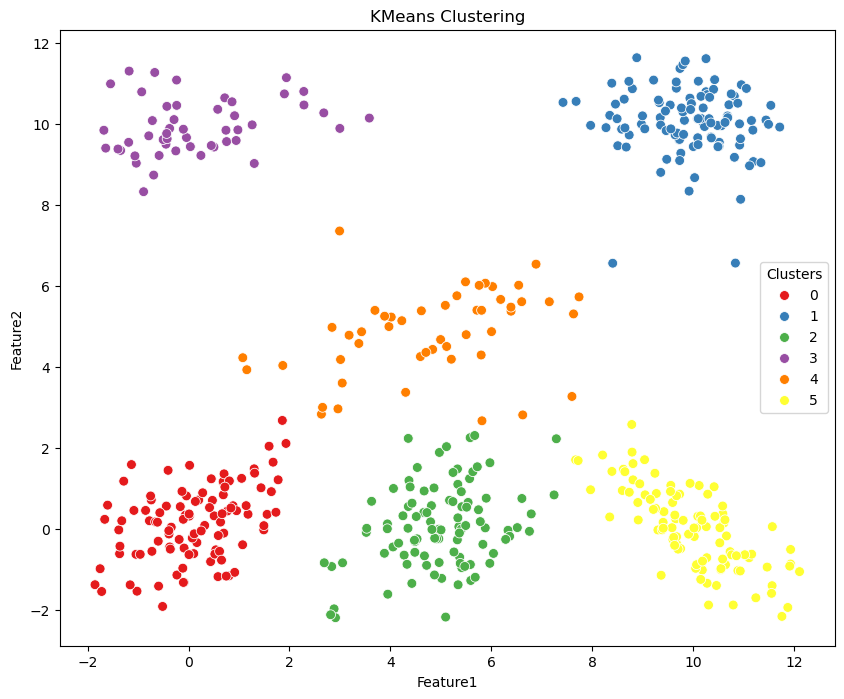
7.1.2 KMeans

KMeans is a clustering method that divides data into K separate clusters, ensuring each data point is assigned to the cluster whose mean (centroid) is closest, determined by its features.

from sklearn.cluster import KMeans
# Define the parameters for KMeans
kmeans = KMeans(n_clusters=6, random_state=50)
# KMeans fitting
kmeans.fit(df[['Feature1', 'Feature2']])
# Generating labels
kmeans_labels = kmeans.predict(df[['Feature1', 'Feature2']])
# Assign the labels of clusters to df
df['kmeans_labels'] = kmeans_labels

# Plot the data with clusters
plt.figure(figsize=(10, 8))
g = sns.scatterplot(data=df, x='Feature1', y='Feature2', hue='kmeans_labels', palette='Set1', s=50, legend=True)
g.set_title('KMeans Clustering')
g.legend(title='Clusters', loc='center right')
plt.show()

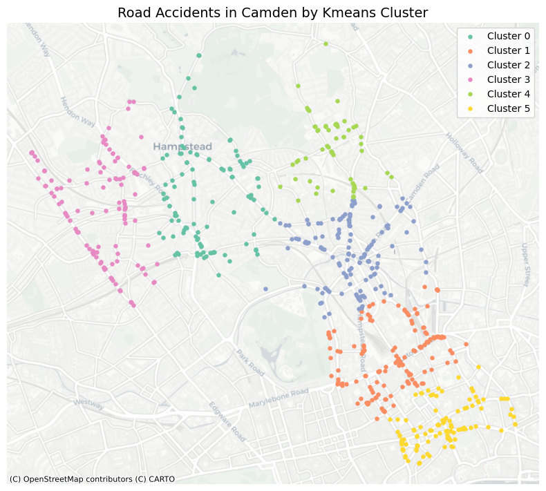
Applying KMeans clustering on road accidents

# KMeans clustering on road accidents in Camden Town
kmeans = KMeans(n_clusters=6, random_state=50)
# KMeans fitting
kmeans.fit(df_accident_camden[['location_easting_osgr', 'location_northing_osgr']])
# Generating labels
kmeans_labels = kmeans.predict(df_accident_camden[['location_easting_osgr', 'location_northing_osgr']])
# put the labels to the df and gdf
df_accident_camden['kmeans_labels'] = kmeans_labels
gdf['kmeans_labels'] = kmeans_labels

# Plot the data with clusters
fig, ax = plt.subplots(figsize=(8, 8))
for label in sorted(gdf['kmeans_labels'].unique()):
    gdf[gdf['kmeans_labels'] == label].plot(
        ax=ax,
        markersize=13,
        color=hex_colors[label],
        label=f"Cluster {label}"
    )

# Add basemap (CartoDB Positron)
ctx.add_basemap(ax, source=ctx.providers.CartoDB.Positron)

# plot
ax.set_axis_off()
plt.legend()
plt.title("Road Accidents in Camden by Kmeans Cluster", fontsize=14)
plt.tight_layout()
plt.show()

7.1.3 DBSCAN

Density-based spatial clustering of applications with noise is a popular density-based clustering algorithm. Unlike partition-based methods like KMeans, DBSCAN is capable of finding clusters of arbitrary shapes and handling noise in the data.

Key Parameters:

• eps (epsilon): The maximum distance between two points for one to be considered as in the neighborhood of the other.

• min_samples: The number of points (pts) in a neighborhood for a pt to be considered as a core pt (This includes the pt itself).

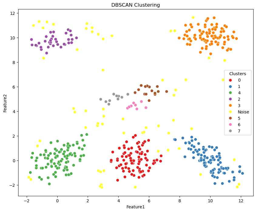
from sklearn.cluster import DBSCAN
# Define the parameters for DBSCAN
dbscan = DBSCAN(eps=0.6, min_samples=5)
# DBSACn implementing
dbscan.fit(df[['Feature1', 'Feature2']])

DBSCAN(eps=0.6)

In a Jupyter environment, please rerun this cell to show the HTML representation or trust the notebook.
On GitHub, the HTML representation is unable to render, please try loading this page with nbviewer.org.

# Generating the labels
df['dbscan_labels'] = dbscan.labels_
print('The numbers of clusters from DBSCAN:', df['dbscan_labels'].nunique()-1)
# We replace -1 with Noise
df.dbscan_labels = df.dbscan_labels.replace({-1:'Noise'})

The numbers of clusters from DBSCAN: 8

# Plot the data with clusters
plt.figure(figsize=(10, 8))
g = sns.scatterplot(data=df, x='Feature1', y='Feature2', hue='dbscan_labels', palette='Set1', s=50, legend=True)
g.set_title('DBSCAN Clustering')
g.legend(title='Clusters', loc='center right')
plt.show()

Applying DBSCAN clustering on road accidents

# Define the parameters for DBSCAN, 200 means in meters, then for each cluster,
# each point is within 200 meters of at least 3 other points.
dbscan = DBSCAN(eps=200, min_samples=3)
# DBSACn implementing
dbscan.fit(df_accident_camden[['location_easting_osgr',
                               'location_northing_osgr']])
# Generating the labels
gdf['dbscan_labels'] = dbscan.labels_
print('The numbers of clusters from DBSCAN:',
      gdf['dbscan_labels'].nunique()-1)

The numbers of clusters from DBSCAN: 25

# define the colors for clusters
palette = sns.color_palette("Set2", n_colors=gdf['dbscan_labels'].nunique()-1)
hex_colors = [mcolors.to_hex(color) for color in palette]
# Plot the data with clusters
fig, ax = plt.subplots(figsize=(8, 8))
for label in sorted(gdf['dbscan_labels'].unique()):
    if label != -1:  # Exclude noise points
        gdf[gdf['dbscan_labels'] == label].plot(
            ax=ax,
            markersize=13,
            color=hex_colors[label],
            label=f"Cluster {label}"
        )
    else:
        gdf[gdf['dbscan_labels'] == label].plot(
            ax=ax,
            markersize=13,
            color='gray',
            label='Noise'
        )
# Add basemap (CartoDB Positron)
ctx.add_basemap(ax, source=ctx.providers.CartoDB.Positron)
# plot
ax.set_axis_off()
plt.legend()
plt.title("Road Accidents in Camden by DBSCAN Cluster", fontsize=14)
plt.tight_layout()
plt.show()

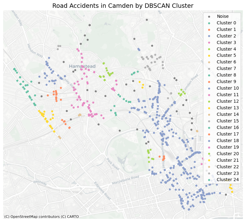
Interpretation:

Though we can see that the clusters from GMM and KMeans are similar, DBSCAN identify more clusters and noise points. This is because DBSCAN is a density-based clustering algorithm, which can find clusters of arbitrary shapes and handle noise in the data. In application, local clusters of road accidents can be identified using DBSCAN, which can help to identify areas with high accident rates and potential hotspots for road safety interventions.

7.2 HyperParameter in clustering

Metrics assess the effectiveness of clustering outcomes. By evaluating various clustering algorithms to select the optimal one or adjusting parameters within the same algorithm for tuning purposes (e.g., selecting the numbers of clusters), we can determine which configuration produces clusters that aligned with our domain knowledge.

Related metrics for clustering in sklearn can be found here

7.2.1 Silhouette coefficient

The Silhouette Coefficient is a metric used to evaluate the quality of clustering in unsupervised learning. It measures how similar each data point is to its own cluster compared to other clusters.

\(s(i) = \frac{b(i) - a(i)}{\max(a(i), b(i))}\)

• \(s(i)\) represents the Silhouette Coefficient for data point \(i\).

• \(a(i)\) is the average distance from to all other points within the same cluster (intra-cluster distance).

• \(b(i)\) is the minimum average distance from i to points in any other cluster (inter-cluster distance).

• \( max(a(i),b(i))\) ensures \(s(i)\) that is normalized to range between -1 and +1.

Interpretation:

• \(s(i)\) near +1 indicates that point \(i\) is well-clustered, with its distance to points in its own cluster significantly smaller than its distance to points in neighboring clusters.

• \(s(i)\) near 0 indicates that point \(i\) is on or very close to the decision boundary between two neighboring clusters.

• \(s(i)\) near -1 indicates that point \(i\) may have been assigned to the wrong cluster.

from sklearn.metrics import silhouette_score

# This function returns the mean Silhouette Coefficient of all samples.
# We calculate the gmm clusters for an example
silhouette_avg = silhouette_score(df[['Feature1', 'Feature2']], df['gmm_labels']) 
print("Silhouette Coefficient:", silhouette_avg)

Silhouette Coefficient: 0.6583554245759751

7.2.2 Davies-Bouldin Index

The Davies-Bouldin Index provides a measure of the average similarity between each cluster.

\( DB = \frac{1}{n} \sum_{i=1}^{n} \max_{j \neq i} \left( \frac{S_i + S_j}{d(c_i, c_j)} \right) \)

• \(n\) is the number of clusters.

• \(S_i\) is the average distance between each point in cluster \(i\) and the centroid \(c_i\).

• \(d(c_i, c_j)\) is the distance between centroids \(c_i\) and \(c_j\).

• \(\max_{j \neq i} \left( \frac{S_i + S_j}{d(c_i, c_j)} \right)\) computes the maximum similarity measure (Euclidean distance) between cluster \(i\) and any other cluster \(j\).

Interpretation:

• Lower values of DB indicate better-defined and well-separated clusters.

from sklearn.metrics import davies_bouldin_score

# Compute Davies-Bouldin Index
# We calculate the gmm clusters for an example
db_index = davies_bouldin_score(df[['Feature1', 'Feature2']], df['gmm_labels'])
print("Davies-Bouldin Index:", db_index)

Davies-Bouldin Index: 0.5099268217594325

7.2.3 Parameter tuning process

Example: optimising the numbers of clusters using Silhouette Scores and DB index in GMM

# Define the range for the number of clusters
cluster_range = range(2, 11)

# Initialize lists to store metric scores
silhouette_scores = []
davies_bouldin_scores = []

for n_clusters in cluster_range:
    # Fit GMM model using different cluster numbers
    gmm = GaussianMixture(n_components=n_clusters, random_state=42)
    gmm.fit(df[['Feature1', 'Feature2']])
    
    # Generating labels
    labels = gmm.predict(df[['Feature1', 'Feature2']])
    
    # Calculate Silhouette Coefficient
    silhouette_avg = silhouette_score(df[['Feature1', 'Feature2']], labels)
    silhouette_scores.append(silhouette_avg)
    
    # Calculate Davies-Bouldin Index
    db_index = davies_bouldin_score(df[['Feature1', 'Feature2']], labels)
    davies_bouldin_scores.append(db_index)
    
    print(f'Number of clusters: {n_clusters}')
    print(f'Silhouette Coefficient: {silhouette_avg}')
    print(f'Davies-Bouldin Index: {db_index}\n')

Number of clusters: 2
Silhouette Coefficient: 0.4759573267675314
Davies-Bouldin Index: 0.9428541532461406

Number of clusters: 3
Silhouette Coefficient: 0.49528077888296457
Davies-Bouldin Index: 0.7161162630982991

Number of clusters: 4
Silhouette Coefficient: 0.5615867904177323
Davies-Bouldin Index: 0.5269555531806575

Number of clusters: 5
Silhouette Coefficient: 0.6167432592503065
Davies-Bouldin Index: 0.5778207829980668

Number of clusters: 6
Silhouette Coefficient: 0.6583554245759751
Davies-Bouldin Index: 0.5099268217594325

Number of clusters: 7
Silhouette Coefficient: 0.582565242046876
Davies-Bouldin Index: 0.5994514303332313

Number of clusters: 8
Silhouette Coefficient: 0.5642378840860819
Davies-Bouldin Index: 0.7263834300455105

Number of clusters: 9
Silhouette Coefficient: 0.5271595593685239
Davies-Bouldin Index: 1.0159927193940836

Number of clusters: 10
Silhouette Coefficient: 0.5212884507182589
Davies-Bouldin Index: 0.983680222721036

# Plotting the metrics with cluster numbers
fig, ax = plt.subplots(1, 2, figsize=(12, 6))
sns.lineplot(x=cluster_range, y=silhouette_scores, marker='o', size=20, ax=ax[0], legend=False)
ax[0].set_title('Silhouette Coefficient')
ax[0].set_xlabel('Number of clusters')
ax[0].set_ylabel('Silhouette Coefficient')

sns.lineplot(x=cluster_range, y=davies_bouldin_scores, marker='o', size=20 ,ax=ax[1], legend=False)
ax[1].set_title('Davies-Bouldin Index')
ax[1].set_xlabel('Number of clusters')
ax[1].set_ylabel('Davies-Bouldin Index')
plt.show()

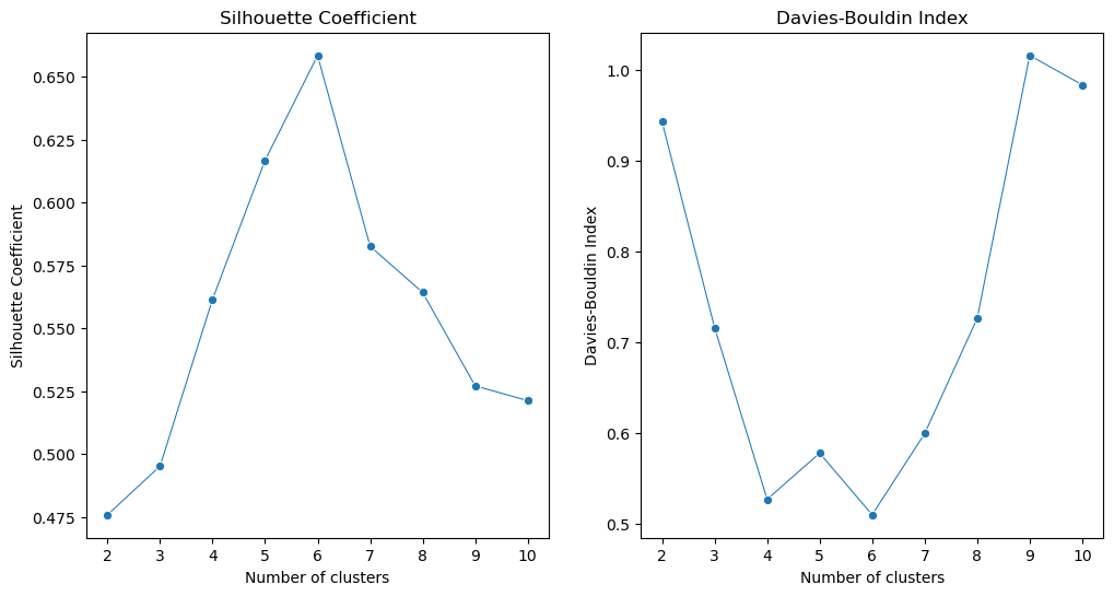
In summary, we can identify the optimal cluster number (6) in this clustering task where the Silhouette Coefficient is highest and the Davies-Bouldin Index is lowest.

The selection of numbers of clusters in DBSCAN clustering:

In DBSCAN, using the index may not get the optimal numbers of clusters as the DB index and Silhouette Coefficient cannot reach the lowest or highest values. For lots of cases, the numbers of clusters in DBSCAN are determined by the domain knowledge and the parameters of DBSCAN, such as eps and min_samples. For example, 500 m is a reasonable distance for some urban analysis as 500 meters is a reasonable distance for people to walk (or around a place) so can be represented for some clustering in urban analysis.

7.3 Spatial and Temporal Clustering

Spatial and temporal clustering combines spatial and temporal dimensions to analyze data that varies over both space and time. This approach is particularly useful in applications such as environmental monitoring, traffic analysis, and social media trend analysis, where data points are not only located in space but also change over time.

For example, for human mobility data, we can cluster the data based on both spatial and temporal dimensions to identify patterns of human movement in a specific area over time. This can help to understand how people move in and out of an area, how long they stay, and how their movement patterns change over time. Or in crime science, the spatial and temporal clustering can be used to identify the near repeat patterns of crime, which can help to understand the patterns of crime in a specific area over time (ref paper).

ST-DBSCAN

Spatio-Temporal Density-Based Spatial Clustering of Applications with Noise. It’s an extension of the classic DBSCAN clustering algorithm designed specifically for spatio-temporal data — that is, data with both spatial (location) and temporal (time) components.

• eps1: Spatial distance threshold (like radius in regular DBSCAN).

• eps2: Temporal distance threshold.

• minPts: Minimum number of points needed to form a dense region.

You can find the ST-DBSCAN doc here

We will use the mobile phone GPS data to identify the visiting behavior from the spatial and temporal patterns of human mobility using ST-DBSCAN. The data is from GeoLife GPS Trajectories. This GPS trajectory dataset was collected in the (Microsoft Research Asia) Geolife project by 182 users in a period of over three years (from April 2007 to August 2012).

# Read the all gps points from 001 user
import glob
path = 'data/Geolife Trajectories 1.3/Data/001/Trajectory/*.plt'
all_files = glob.glob(path)
all_files.sort()  # Sort the files to ensure they are in order
print(len(all_files), all_files)

71 ['data/Geolife Trajectories 1.3/Data/001/Trajectory/20081023055305.plt', 'data/Geolife Trajectories 1.3/Data/001/Trajectory/20081023234104.plt', 'data/Geolife Trajectories 1.3/Data/001/Trajectory/20081024234405.plt', 'data/Geolife Trajectories 1.3/Data/001/Trajectory/20081025231428.plt', 'data/Geolife Trajectories 1.3/Data/001/Trajectory/20081026081229.plt', 'data/Geolife Trajectories 1.3/Data/001/Trajectory/20081027111634.plt', 'data/Geolife Trajectories 1.3/Data/001/Trajectory/20081027233029.plt', 'data/Geolife Trajectories 1.3/Data/001/Trajectory/20081027235802.plt', 'data/Geolife Trajectories 1.3/Data/001/Trajectory/20081028102805.plt', 'data/Geolife Trajectories 1.3/Data/001/Trajectory/20081028233053.plt', 'data/Geolife Trajectories 1.3/Data/001/Trajectory/20081028235048.plt', 'data/Geolife Trajectories 1.3/Data/001/Trajectory/20081029110529.plt', 'data/Geolife Trajectories 1.3/Data/001/Trajectory/20081029234123.plt', 'data/Geolife Trajectories 1.3/Data/001/Trajectory/20081030233959.plt', 'data/Geolife Trajectories 1.3/Data/001/Trajectory/20081101004235.plt', 'data/Geolife Trajectories 1.3/Data/001/Trajectory/20081102030834.plt', 'data/Geolife Trajectories 1.3/Data/001/Trajectory/20081102233452.plt', 'data/Geolife Trajectories 1.3/Data/001/Trajectory/20081103133204.plt', 'data/Geolife Trajectories 1.3/Data/001/Trajectory/20081103233729.plt', 'data/Geolife Trajectories 1.3/Data/001/Trajectory/20081104054859.plt', 'data/Geolife Trajectories 1.3/Data/001/Trajectory/20081104234436.plt', 'data/Geolife Trajectories 1.3/Data/001/Trajectory/20081105110052.plt', 'data/Geolife Trajectories 1.3/Data/001/Trajectory/20081106051423.plt', 'data/Geolife Trajectories 1.3/Data/001/Trajectory/20081106133604.plt', 'data/Geolife Trajectories 1.3/Data/001/Trajectory/20081106233404.plt', 'data/Geolife Trajectories 1.3/Data/001/Trajectory/20081108034358.plt', 'data/Geolife Trajectories 1.3/Data/001/Trajectory/20081109033335.plt', 'data/Geolife Trajectories 1.3/Data/001/Trajectory/20081110233534.plt', 'data/Geolife Trajectories 1.3/Data/001/Trajectory/20081111114304.plt', 'data/Geolife Trajectories 1.3/Data/001/Trajectory/20081111234235.plt', 'data/Geolife Trajectories 1.3/Data/001/Trajectory/20081112234504.plt', 'data/Geolife Trajectories 1.3/Data/001/Trajectory/20081113121334.plt', 'data/Geolife Trajectories 1.3/Data/001/Trajectory/20081113234558.plt', 'data/Geolife Trajectories 1.3/Data/001/Trajectory/20081114130723.plt', 'data/Geolife Trajectories 1.3/Data/001/Trajectory/20081115003535.plt', 'data/Geolife Trajectories 1.3/Data/001/Trajectory/20081116024429.plt', 'data/Geolife Trajectories 1.3/Data/001/Trajectory/20081116235322.plt', 'data/Geolife Trajectories 1.3/Data/001/Trajectory/20081117042454.plt', 'data/Geolife Trajectories 1.3/Data/001/Trajectory/20081117234459.plt', 'data/Geolife Trajectories 1.3/Data/001/Trajectory/20081118003844.plt', 'data/Geolife Trajectories 1.3/Data/001/Trajectory/20081118132804.plt', 'data/Geolife Trajectories 1.3/Data/001/Trajectory/20081118235053.plt', 'data/Geolife Trajectories 1.3/Data/001/Trajectory/20081119104736.plt', 'data/Geolife Trajectories 1.3/Data/001/Trajectory/20081120121822.plt', 'data/Geolife Trajectories 1.3/Data/001/Trajectory/20081120234905.plt', 'data/Geolife Trajectories 1.3/Data/001/Trajectory/20081201102704.plt', 'data/Geolife Trajectories 1.3/Data/001/Trajectory/20081202000605.plt', 'data/Geolife Trajectories 1.3/Data/001/Trajectory/20081202145929.plt', 'data/Geolife Trajectories 1.3/Data/001/Trajectory/20081203000505.plt', 'data/Geolife Trajectories 1.3/Data/001/Trajectory/20081203112659.plt', 'data/Geolife Trajectories 1.3/Data/001/Trajectory/20081203235305.plt', 'data/Geolife Trajectories 1.3/Data/001/Trajectory/20081204142253.plt', 'data/Geolife Trajectories 1.3/Data/001/Trajectory/20081205002359.plt', 'data/Geolife Trajectories 1.3/Data/001/Trajectory/20081205143505.plt', 'data/Geolife Trajectories 1.3/Data/001/Trajectory/20081205235730.plt', 'data/Geolife Trajectories 1.3/Data/001/Trajectory/20081206040725.plt', 'data/Geolife Trajectories 1.3/Data/001/Trajectory/20081206083854.plt', 'data/Geolife Trajectories 1.3/Data/001/Trajectory/20081206084030.plt', 'data/Geolife Trajectories 1.3/Data/001/Trajectory/20081207030135.plt', 'data/Geolife Trajectories 1.3/Data/001/Trajectory/20081208001534.plt', 'data/Geolife Trajectories 1.3/Data/001/Trajectory/20081208142853.plt', 'data/Geolife Trajectories 1.3/Data/001/Trajectory/20081209002004.plt', 'data/Geolife Trajectories 1.3/Data/001/Trajectory/20081210001529.plt', 'data/Geolife Trajectories 1.3/Data/001/Trajectory/20081210080559.plt', 'data/Geolife Trajectories 1.3/Data/001/Trajectory/20081210235522.plt', 'data/Geolife Trajectories 1.3/Data/001/Trajectory/20081211110523.plt', 'data/Geolife Trajectories 1.3/Data/001/Trajectory/20081212000534.plt', 'data/Geolife Trajectories 1.3/Data/001/Trajectory/20081212141923.plt', 'data/Geolife Trajectories 1.3/Data/001/Trajectory/20081213092204.plt', 'data/Geolife Trajectories 1.3/Data/001/Trajectory/20081214080334.plt', 'data/Geolife Trajectories 1.3/Data/001/Trajectory/20081214235553.plt']

# read all files and concatenate them into a single DataFrame
df_geolife = pd.concat((pd.read_csv(f, header=None, skiprows=6) for f in all_files), ignore_index=True)

# the df includes spatial and temporal information
df_geolife

	0	1	2	3	4	5	6
0	39.984094	116.319236	0	492	39744.245197	2008-10-23	05:53:05
1	39.984198	116.319322	0	492	39744.245208	2008-10-23	05:53:06
2	39.984224	116.319402	0	492	39744.245266	2008-10-23	05:53:11
3	39.984211	116.319389	0	492	39744.245324	2008-10-23	05:53:16
4	39.984217	116.319422	0	491	39744.245382	2008-10-23	05:53:21
...	...	...	...	...	...	...	...
108602	39.977969	116.326651	0	311	39797.021505	2008-12-15	00:30:58
108603	39.977946	116.326653	0	310	39797.021562	2008-12-15	00:31:03
108604	39.977897	116.326624	0	310	39797.021620	2008-12-15	00:31:08
108605	39.977882	116.326626	0	310	39797.021678	2008-12-15	00:31:13
108606	39.977879	116.326628	0	310	39797.021736	2008-12-15	00:31:18

108607 rows × 7 columns

# add column names
df_geolife.columns = ['Latitude', 'Longitude', '2', 'Altitude', '4', 'Date', 'Time']
# astype
df_geolife['Date'] = df_geolife['Date'].astype(str)
df_geolife['Time'] = df_geolife['Time'].astype(str)
# combine date and time into a single datetime column
df_geolife['Datetime'] = pd.to_datetime(df_geolife['Date'] + ' ' + df_geolife['Time'], format='%Y-%m-%d %H:%M:%S')

df_geolife['Date'].unique()

array(['2008-10-23', '2008-10-24', '2008-10-25', '2008-10-26',
       '2008-10-27', '2008-10-28', '2008-10-29', '2008-10-30',
       '2008-10-31', '2008-11-01', '2008-11-02', '2008-11-03',
       '2008-11-04', '2008-11-05', '2008-11-06', '2008-11-07',
       '2008-11-08', '2008-11-09', '2008-11-10', '2008-11-11',
       '2008-11-12', '2008-11-13', '2008-11-14', '2008-11-15',
       '2008-11-16', '2008-11-17', '2008-11-18', '2008-11-19',
       '2008-11-20', '2008-11-21', '2008-12-01', '2008-12-02',
       '2008-12-03', '2008-12-04', '2008-12-05', '2008-12-06',
       '2008-12-07', '2008-12-08', '2008-12-09', '2008-12-10',
       '2008-12-11', '2008-12-12', '2008-12-13', '2008-12-14',
       '2008-12-15'], dtype=object)

df_geolife = df_geolife[['Latitude', 'Longitude', 'Altitude', 'Datetime']]

gdf_geolife = gpd.GeoDataFrame(df_geolife, geometry=gpd.points_from_xy(df_geolife['Longitude'], df_geolife['Latitude']), crs="EPSG:4326")
print(gdf_geolife.crs)

EPSG:4326

gdf_geolife

	Latitude	Longitude	Altitude	Datetime	geometry
0	39.984094	116.319236	492	2008-10-23 05:53:05	POINT (116.31924 39.98409)
1	39.984198	116.319322	492	2008-10-23 05:53:06	POINT (116.31932 39.9842)
2	39.984224	116.319402	492	2008-10-23 05:53:11	POINT (116.3194 39.98422)
3	39.984211	116.319389	492	2008-10-23 05:53:16	POINT (116.31939 39.98421)
4	39.984217	116.319422	491	2008-10-23 05:53:21	POINT (116.31942 39.98422)
...	...	...	...	...	...
108602	39.977969	116.326651	311	2008-12-15 00:30:58	POINT (116.32665 39.97797)
108603	39.977946	116.326653	310	2008-12-15 00:31:03	POINT (116.32665 39.97795)
108604	39.977897	116.326624	310	2008-12-15 00:31:08	POINT (116.32662 39.9779)
108605	39.977882	116.326626	310	2008-12-15 00:31:13	POINT (116.32663 39.97788)
108606	39.977879	116.326628	310	2008-12-15 00:31:18	POINT (116.32663 39.97788)

108607 rows × 5 columns

import folium
m = folium.Map(location=[39.989614, 116.327158], zoom_start=12, tiles='CartoDB Positron')
# only show the 2008-10-28 points for better visualization
gdf_geolife_sample = gdf_geolife[gdf_geolife['Datetime'].dt.date == pd.to_datetime('2008-10-28').date()]
# As there are too many points, we use samples to plot the points
for _, row in gdf_geolife_sample.iterrows():
    folium.CircleMarker(
        location=[row.geometry.y, row.geometry.x],
        radius=1,
        color='RoyalBlue',
        fill=True,
        fill_color='RoyalBlue',
        fill_opacity=0.8
    ).add_to(m)
m

Make this Notebook Trusted to load map: File -> Trust Notebook

We use ST-DBSCAN to cluster the data, as DBSCAN is not suitable for spatio-temporal data. If we set the eps for spatial and temporal units, a ST-cluster represents a group of points that an individual moves within a certain distance and certain time around a place. So this can be used to detect human activities at places in urban analytics. For example, if we set 50 meters and 5 minutes, a ST-cluster represents the user moves within 10 meters and 5 minutes around a place. Such a cluster can be used to identify the stay points of the user. Or for GPS data, we can infer the travel mode from this, like walking, cycling, or driving. For GPS of Cars, We can infer the traffic jams or traffic flow from the clusters.

# pip install st-dbscan

import st_dbscan

# we need to transfer the data to projected coordinates, as this is in lat/lon and in Beijing, China, we can UTM Zone 50N projection
gdf_geolife_sample_p = gdf_geolife_sample.to_crs("EPSG:32650")
gdf_geolife_sample_p

	Latitude	Longitude	Altitude	Datetime	geometry
18430	39.978943	116.325146	392	2008-10-28 00:00:38	POINT (442376.74 4425638.146)
18431	39.978928	116.325205	406	2008-10-28 00:00:43	POINT (442381.765 4425636.443)
18432	39.978911	116.325194	414	2008-10-28 00:00:48	POINT (442380.811 4425634.563)
18433	39.979037	116.325211	422	2008-10-28 00:01:13	POINT (442382.369 4425648.537)
18434	39.978904	116.325214	410	2008-10-28 00:01:14	POINT (442382.513 4425633.773)
...	...	...	...	...	...
19621	39.982950	116.326545	1817	2008-10-28 23:59:22	POINT (442499.555 4426081.984)
19622	39.982934	116.326552	1818	2008-10-28 23:59:27	POINT (442500.139 4426080.204)
19623	39.982920	116.326564	1818	2008-10-28 23:59:32	POINT (442501.152 4426078.642)
19624	39.982920	116.326564	1818	2008-10-28 23:59:35	POINT (442501.152 4426078.642)
19625	39.982913	116.326569	1818	2008-10-28 23:59:37	POINT (442501.573 4426077.862)

1196 rows × 5 columns

# we create a x and y column for the projected coordinates
gdf_geolife_sample_p['x'] = gdf_geolife_sample_p.geometry.x
gdf_geolife_sample_p['y'] = gdf_geolife_sample_p.geometry.y

gdf_geolife_sample_p

	Latitude	Longitude	Altitude	Datetime	geometry	x	y
18430	39.978943	116.325146	392	2008-10-28 00:00:38	POINT (442376.74 4425638.146)	442376.739518	4.425638e+06
18431	39.978928	116.325205	406	2008-10-28 00:00:43	POINT (442381.765 4425636.443)	442381.764750	4.425636e+06
18432	39.978911	116.325194	414	2008-10-28 00:00:48	POINT (442380.811 4425634.563)	442380.811214	4.425635e+06
18433	39.979037	116.325211	422	2008-10-28 00:01:13	POINT (442382.369 4425648.537)	442382.368622	4.425649e+06
18434	39.978904	116.325214	410	2008-10-28 00:01:14	POINT (442382.513 4425633.773)	442382.513075	4.425634e+06
...	...	...	...	...	...	...	...
19621	39.982950	116.326545	1817	2008-10-28 23:59:22	POINT (442499.555 4426081.984)	442499.554866	4.426082e+06
19622	39.982934	116.326552	1818	2008-10-28 23:59:27	POINT (442500.139 4426080.204)	442500.139127	4.426080e+06
19623	39.982920	116.326564	1818	2008-10-28 23:59:32	POINT (442501.152 4426078.642)	442501.151975	4.426079e+06
19624	39.982920	116.326564	1818	2008-10-28 23:59:35	POINT (442501.152 4426078.642)	442501.151975	4.426079e+06
19625	39.982913	116.326569	1818	2008-10-28 23:59:37	POINT (442501.573 4426077.862)	442501.573017	4.426078e+06

1196 rows × 7 columns

# We need to caculate each point's speed, which can help to identify the stay points or walking points.
# We can use the difference of time and distance to calculate the speed

# Calculate the time difference in seconds
gdf_geolife_sample_p['time_diff'] = gdf_geolife_sample_p['Datetime'].diff().dt.total_seconds().fillna(0)

# Calculate distance between consecutive points
gdf_geolife_sample_p['distance'] = gdf_geolife_sample_p.geometry.distance(gdf_geolife_sample_p.geometry.shift()).fillna(0)

# Calculate speed (meters per second)
gdf_geolife_sample_p['speed'] = gdf_geolife_sample_p['distance'] / gdf_geolife_sample_p['time_diff']

# Filter for slow (likely stationary or walking) points
gdf_geolife_sample_slow = gdf_geolife_sample_p[gdf_geolife_sample_p['speed'] < 2]

gdf_geolife_sample_slow

	Latitude	Longitude	Altitude	Datetime	geometry	x	y	time_diff	distance	speed
18431	39.978928	116.325205	406	2008-10-28 00:00:43	POINT (442381.765 4425636.443)	442381.764750	4.425636e+06	5.0	5.305953	1.061191
18432	39.978911	116.325194	414	2008-10-28 00:00:48	POINT (442380.811 4425634.563)	442380.811214	4.425635e+06	5.0	2.107762	0.421552
18433	39.979037	116.325211	422	2008-10-28 00:01:13	POINT (442382.369 4425648.537)	442382.368622	4.425649e+06	25.0	14.060423	0.562417
18436	39.978802	116.325175	398	2008-10-28 00:01:22	POINT (442379.097 4425622.477)	442379.097307	4.425622e+06	5.0	1.334667	0.266933
18437	39.978815	116.325199	394	2008-10-28 00:01:27	POINT (442381.158 4425623.904)	442381.157517	4.425624e+06	5.0	2.506366	0.501273
...	...	...	...	...	...	...	...	...	...	...
19621	39.982950	116.326545	1817	2008-10-28 23:59:22	POINT (442499.555 4426081.984)	442499.554866	4.426082e+06	5.0	2.849030	0.569806
19622	39.982934	116.326552	1818	2008-10-28 23:59:27	POINT (442500.139 4426080.204)	442500.139127	4.426080e+06	5.0	1.873791	0.374758
19623	39.982920	116.326564	1818	2008-10-28 23:59:32	POINT (442501.152 4426078.642)	442501.151975	4.426079e+06	5.0	1.861318	0.372264
19624	39.982920	116.326564	1818	2008-10-28 23:59:35	POINT (442501.152 4426078.642)	442501.151975	4.426079e+06	3.0	0.000000	0.000000
19625	39.982913	116.326569	1818	2008-10-28 23:59:37	POINT (442501.573 4426077.862)	442501.573017	4.426078e+06	2.0	0.886527	0.443264

287 rows × 10 columns

# set the unix time
gdf_geolife_sample_slow['unixtime'] = gdf_geolife_sample_slow['Datetime'].astype(np.int64) // 10**9
# we use ST-DBSCAN to cluster the data, eps is in meters, and min_samples is in seconds
st_dbscan_model = st_dbscan.ST_DBSCAN(eps1=20, eps2=5*60, min_samples=5)  # eps in meters, min_samples in seconds
# fit the model
st_dbscan_model.fit(gdf_geolife_sample_slow[['x', 'y', 'unixtime']])

<st_dbscan.st_dbscan.ST_DBSCAN at 0x1711cd720>

st_dbscan_model.labels

array([-1, -1, -1,  0,  0,  0,  0,  0, -1, -1, -1, -1,  1,  1,  1,  1,  1,
        1,  1, -1, -1, -1, -1, -1, -1, -1, -1, -1,  2,  2,  2,  2,  2,  2,
        2,  2,  2,  2,  2, -1, -1, -1, -1,  3,  3,  3,  3,  3,  3,  3,  3,
       -1, -1, -1,  4,  4,  4,  4,  4,  4,  4,  4,  4, -1, -1, -1, -1, -1,
       -1,  5,  5,  5,  5,  5,  5,  5,  5,  5,  5,  5,  5,  5,  5,  5,  5,
        5,  5,  5, -1, -1, -1, -1, -1,  6,  6,  6,  6,  6,  6,  6,  6,  6,
        6,  6,  6,  6,  6,  6,  6,  6,  7,  7,  7,  7,  7,  7,  7,  7,  7,
        7,  7,  7,  7, -1, -1, -1, -1, -1, -1,  8,  8,  8,  8,  8,  8,  8,
        8,  8,  8,  8, -1,  9,  9,  9,  9,  9,  9, -1, -1, 10, 10, 10, 10,
       10, 10, 10, -1, 11, 11, 11, 11, 11, -1, -1, -1, -1, -1, -1, -1, 12,
       12, 12, 12, 12, 12, 12, 12, 12, 12, 12, 12, 12, -1, -1, 13, 13, 13,
       13, 13, 13, 13, 13, 13, 13, 13, 13, 13, 13, 13, -1, -1, -1, -1, 14,
       14, 14, 14, 14, 14, 14, -1, -1, -1, -1, -1, -1, -1, -1, -1, -1, -1,
       15, 15, 15, 15, 15, -1, -1, -1, 16, 16, 16, 16, 16, -1, -1, -1, -1,
       -1, 17, 17, 17, 17, 17, -1, 18, 18, 18, 18, 18, 18, 18, 18, 18, 18,
       -1, -1, -1, -1, -1, -1, -1, -1, -1, -1, 19, 19, 19, 19, 19, 19, 19,
       19, 20, 20, 20, 20, 20, 20, 20, 20, 20, 20, 20, 20, 20, 20])

gdf_geolife_sample_slow['labels'] = st_dbscan_model.labels

gdf_geolife_sample_slow.labels.value_counts()

labels
-1     87
 5     19
 6     17
 13    15
 20    14
 12    13
 7     13
 2     11
 8     11
 18    10
 4      9
 3      8
 19     8
 1      7
 14     7
 10     7
 9      6
 0      5
 11     5
 15     5
 16     5
 17     5
Name: count, dtype: int64

gdf_geolife_sample_slow['labels'].nunique()

22

gdf_geolife_sample_slow

	Latitude	Longitude	Altitude	Datetime	geometry	x	y	time_diff	distance	speed	unixtime	labels
18431	39.978928	116.325205	406	2008-10-28 00:00:43	POINT (442381.765 4425636.443)	442381.764750	4.425636e+06	5.0	5.305953	1.061191	1225152043	-1
18432	39.978911	116.325194	414	2008-10-28 00:00:48	POINT (442380.811 4425634.563)	442380.811214	4.425635e+06	5.0	2.107762	0.421552	1225152048	-1
18433	39.979037	116.325211	422	2008-10-28 00:01:13	POINT (442382.369 4425648.537)	442382.368622	4.425649e+06	25.0	14.060423	0.562417	1225152073	-1
18436	39.978802	116.325175	398	2008-10-28 00:01:22	POINT (442379.097 4425622.477)	442379.097307	4.425622e+06	5.0	1.334667	0.266933	1225152082	0
18437	39.978815	116.325199	394	2008-10-28 00:01:27	POINT (442381.158 4425623.904)	442381.157517	4.425624e+06	5.0	2.506366	0.501273	1225152087	0
...	...	...	...	...	...	...	...	...	...	...	...	...
19621	39.982950	116.326545	1817	2008-10-28 23:59:22	POINT (442499.555 4426081.984)	442499.554866	4.426082e+06	5.0	2.849030	0.569806	1225238362	20
19622	39.982934	116.326552	1818	2008-10-28 23:59:27	POINT (442500.139 4426080.204)	442500.139127	4.426080e+06	5.0	1.873791	0.374758	1225238367	20
19623	39.982920	116.326564	1818	2008-10-28 23:59:32	POINT (442501.152 4426078.642)	442501.151975	4.426079e+06	5.0	1.861318	0.372264	1225238372	20
19624	39.982920	116.326564	1818	2008-10-28 23:59:35	POINT (442501.152 4426078.642)	442501.151975	4.426079e+06	3.0	0.000000	0.000000	1225238375	20
19625	39.982913	116.326569	1818	2008-10-28 23:59:37	POINT (442501.573 4426077.862)	442501.573017	4.426078e+06	2.0	0.886527	0.443264	1225238377	20

287 rows × 12 columns

from matplotlib.colors import rgb2hex

# Define and convert palette (excluding noise)
unique_labels = sorted(gdf_geolife_sample_slow['labels'].unique())
non_noise_labels = [label for label in unique_labels if label != -1]

palette_rgb = sns.color_palette("Set2", n_colors=len(non_noise_labels))
palette_hex = [rgb2hex(color) for color in palette_rgb]

# Map labels to colors
label_to_color = {label: palette_hex[i] for i, label in enumerate(non_noise_labels)}
label_to_color[-1] = 'black'  # Noise points as black

# Create the map
m = folium.Map(location=[39.989614, 116.327158], zoom_start=14, tiles='CartoDB Positron')

# Plot all points with correct colors
for _, row in gdf_geolife_sample_slow.iterrows():
    label = row['labels']
    folium.CircleMarker(
        location=[row.Latitude, row.Longitude],
        radius=2,
        color=label_to_color[label],
        fill=True,
        fill_color=label_to_color[label],
        fill_opacity=0.8,
        popup=f"Cluster {label}" if label != -1 else "Noise"
    ).add_to(m)

# Build the legend HTML manually
legend_html = """
<div style="
    position: fixed;
    bottom: 50px; left: 50px; width: 180px; height: auto;
    background-color: white;
    border:2px solid grey;
    z-index:9999;
    font-size:14px;
    padding: 10px;
    box-shadow: 2px 2px 5px rgba(0,0,0,0.3);
">
<b>Legend</b><br>
"""

# Add entries for each label
for label in label_to_color:
    color = label_to_color[label]
    label_name = f"Cluster {label}" if label != -1 else "Noise"
    legend_html += f'<i style="background:{color}; width:10px; height:10px; display:inline-block; margin-right:5px;"></i>{label_name}<br>'

legend_html += "</div>"

# Add the legend to the map
m.get_root().html.add_child(folium.Element(legend_html))

m

Make this Notebook Trusted to load map: File -> Trust Notebook

Quiz

• Q1: For road accident data, identify the clusters of road accidents in HUll city (use local_authority_ons_district == 'E06000010'), use the DBSCAN to detect the local clusters (eps = 50m).

• Q2: Plot the clusters on the interactive map.

• Q3: Output the cluster’s attribute distribution, like accident_severity. All the schema info can be found in data/dft-road-casualty-statistics-road-safety-open-dataset-data-guide-2024.xlsx

Q1 solution

# select the road accident data in Hull city
df_accident_hull = df_accident[df_accident.local_authority_ons_district == 'E06000010']

# we can use the eps = 100m and min_samples = 3 to detect the local clusters
dbscan_hull = DBSCAN(eps=100, min_samples=8)
# DBSCAN implementing
dbscan_hull.fit(df_accident_hull[['location_easting_osgr', 'location_northing_osgr']])
# Generating the labels
df_accident_hull['dbscan_labels'] = dbscan_hull.labels_

# we can see the numbers of clusters are 46
df_accident_hull['dbscan_labels'].nunique()

5

df_accident_hull['dbscan_labels'].value_counts()

dbscan_labels
-1    656
 1     10
 0      9
 2      9
 3      8
Name: count, dtype: int64

Q2 solution

# to plot the clusters on the interactive map, each cluster is represented by a different color
# define the colors for clusters
palette = sns.color_palette("Set1", n_colors=df_accident_hull['dbscan_labels'].nunique()-1)
hex_colors = [mcolors.to_hex(color) for color in palette]
import folium
# Create a map centered around Hull
m_hull = folium.Map(location=[53.7446, -0.3364], zoom_start=13, tiles='CartoDB Positron')
# Add road accidents to the map
for _, row in df_accident_hull.iterrows():
    if row['dbscan_labels'] != -1:  # Exclude noise points
        folium.CircleMarker(
            location=[row['latitude'], row['longitude']],
            radius=5,
            color=hex_colors[row['dbscan_labels']],
            fill=True,
            fill_color=hex_colors[row['dbscan_labels']],
            fill_opacity=0.8
        ).add_to(m_hull)
    else:
        folium.CircleMarker(
            location=[row['latitude'], row['longitude']],
            radius=1,
            color='gray', # noise points in gray and smaller
            fill=True,
            fill_color='gray',
            fill_opacity=0.8
        ).add_to(m_hull)
m_hull

Make this Notebook Trusted to load map: File -> Trust Notebook

Q3 solution

df_accident_hull

	accident_index	accident_year	accident_reference	location_easting_osgr	location_northing_osgr	longitude	latitude	police_force	accident_severity	number_of_vehicles	...	weather_conditions	road_surface_conditions	special_conditions_at_site	carriageway_hazards	urban_or_rural_area	did_police_officer_attend_scene_of_accident	trunk_road_flag	lsoa_of_accident_location	enhanced_severity_collision	dbscan_labels
42911	2023161259218	2023	161259218	512565.0	430430.0	-0.294088	53.758080	16	3	2	...	1	2	0	0	1	1	2	E01012894	3	-1
42913	2023161259253	2023	161259253	506690.0	428678.0	-0.383764	53.743573	16	3	2	...	1	1	0	0	1	1	2	E01012865	3	-1
42915	2023161259587	2023	161259587	508294.0	427894.0	-0.359728	53.736199	16	2	2	...	4	2	0	0	1	1	2	E01012889	5	-1
42919	2023161259760	2023	161259760	506591.0	431025.0	-0.384456	53.764680	16	2	2	...	1	1	0	0	1	1	2	E01012794	7	-1
42920	2023161259768	2023	161259768	512239.0	429220.0	-0.299469	53.747279	16	3	1	...	1	1	0	0	1	1	1	E01012848	3	-1
...	...	...	...	...	...	...	...	...	...	...	...	...	...	...	...	...	...	...	...	...	...
44870	2023161394255	2023	161394255	510320.0	429252.0	-0.328544	53.747976	16	3	2	...	1	1	0	0	1	3	2	E01012809	3	-1
44871	2023161394288	2023	161394288	509768.0	430438.0	-0.336490	53.758747	16	3	2	...	1	1	0	0	1	2	2	E01012867	3	-1
44872	2023161394309	2023	161394309	507077.0	429479.0	-0.377622	53.750691	16	3	1	...	2	2	0	0	1	1	2	E01012862	3	-1
44874	2023161395038	2023	161395038	512127.0	432042.0	-0.300143	53.772656	16	3	1	...	1	1	0	0	1	1	2	E01012812	3	-1
44876	2023161396602	2023	161396602	510113.0	433789.0	-0.330065	53.788781	16	3	2	...	1	1	0	0	2	2	2	E01012789	3	-1

692 rows × 38 columns

accident_severity = {
    1: "Fatal",
    2: "Serious",
    3: "Slight"
}

for label in df_accident_hull['dbscan_labels'].unique():
    if label != -1:  # Exclude noise points
        cluster_data = df_accident_hull[df_accident_hull['dbscan_labels'] == label]
        severity_counts = cluster_data['accident_severity'].value_counts().to_dict()
        print(f"Cluster {label} severity distribution:")
        for severity, count in severity_counts.items():
            print(f"  {accident_severity[severity]}: {count}")

Cluster 0 severity distribution:
  Serious: 5
  Slight: 4
Cluster 3 severity distribution:
  Slight: 8
Cluster 1 severity distribution:
  Slight: 7
  Serious: 3
Cluster 2 severity distribution:
  Slight: 7
  Serious: 2